Portfolio Construction & Measuring Risk Using the Markowitz Method

This notebook will shed some light on the importance of diversification in investments.

First, using the pandas package, I will review the basic steps for collecting & measuring stock returns, as well as how to measure a portfolio return using specific weights. After that, I will show an example of how one can assess a portfolio's risk level using the Markowitz method, by introducing the concept of return correlations among securities. At the end of this notebook, you will learn how to estimate the risk of a portfolio of stocks.

---

Loading the necessary packages

When using Python, I recommend you make it a habit to load the needed packages for your session at the beginning of your code.

This step is similar to the steps taken in my previous Jupyter Notebook series. However, I will add another important package here: (fredapi). This package is made and managed by the Federal Reserve Bank of St. Louis in the United States. Using the package allows the user to download economic data directly from their server. It is basically a portal one can use to obtain any public data provided by the Fed. In order to use this feature, you are required to first open an account at their website, and then request an *API Key*. From my experience, the API-Key request is approved immediately. Check this link for more info: https://fred.stlouisfed.org/docs/api/api_key.html

# If it is your first time using fredapi, you need to download it to your anaconda library. 
# You can do it through the anaconda program (like what you did with the package yfinance) 
# Or alternatively, run the following code here only once on your computer

%pip install fredapi

Collecting fredapi
  Obtaining dependency information for fredapi from https://files.pythonhosted.org/packages/96/d4/f81fa9f67775a6a4b9e2cd8487239d61a9698cb2b9c02a5a2897d310f7a4/fredapi-0.5.1-py3-none-any.whl.metadata
  Downloading fredapi-0.5.1-py3-none-any.whl.metadata (5.0 kB)
Requirement already satisfied: pandas in /Users/eyad/anaconda3/lib/python3.11/site-packages (from fredapi) (1.5.3)
Requirement already satisfied: python-dateutil>=2.8.1 in /Users/eyad/anaconda3/lib/python3.11/site-packages (from pandas->fredapi) (2.8.2)
Requirement already satisfied: pytz>=2020.1 in /Users/eyad/anaconda3/lib/python3.11/site-packages (from pandas->fredapi) (2022.7)
Requirement already satisfied: numpy>=1.21.0 in /Users/eyad/anaconda3/lib/python3.11/site-packages (from pandas->fredapi) (1.24.3)
Requirement already satisfied: six>=1.5 in /Users/eyad/anaconda3/lib/python3.11/site-packages (from python-dateutil>=2.8.1->pandas->fredapi) (1.16.0)
Downloading fredapi-0.5.1-py3-none-any.whl (11 kB)
Installing collected packages: fredapi
Successfully installed fredapi-0.5.1

# Use the package fredapi if you have installed it
from fredapi import Fred
# Don't forget to use your api-key after opening account with FRED
# So then you can download any data from their server
fred = Fred(api_key = '44303cd2e2752fc88d6080b1e0d9d1e9')

# Download the same libraries we used in the past
import yfinance as yf, pandas as pd, datetime as dt, matplotlib as mpl, matplotlib.pyplot as plt

# This library is helpful to use for many math applications, such as matrix multiplication and 
# creating random numbers
import numpy as np

---

Collecting Monthly Returns

Let us use the package yfinance to download monthly prices (so I can measure monthly returns) for the same list of stocks:

["BA", "AMZN", "CVX", "DIS", "GOLD", "HSY", "INTC", "K", "KO", "M", "MMM", "MSFT", "NVDA"].

For a later comparison, I would like to download historical data on an index that hopefully represents the performance of the overall market during the same period. One appropriate option is the Wilshire 5000 Total Market Index, it's ticker in yfinance is ^W5000.

Furthermore, I would like to obtain data on historical T-bills so I can measure the risk-free rate ($R_{f}$). T-bill monthly returns data will be obtained from FRED. The code used by FRED for the 4-week-maturity treasury bill is TB4WK. If I am working with annual or daily stock returns for example, I probably will need to download something different from FRED. This is because the risk-free rate has to be for the same investment horizon I am analyzing. (In my case it is monthly)

Recall the U.S. Federal Reserve Bank sells T-bill securities that have different maturities during the same time; 4, 13, 26, and 52 weeks. Ideally, I would like to measure the return on a T-bill investment that has a maturity matching my investment horizon (Again, for my analysis its 1 month). So for example if I am examining the return of AMZN during the month of April 2016, I would like to compare the stock's performance with a T-bill security that was issued by the fed at the beginning of April 2016 and has a maturity of 1 month.

But what if there are no T-bills sold by the Federal Bank that has a maturity matching my investment horizon? Say if my investment horizon is 1 week, what can I do?

Well, to answer this question, remember that T-bills are money market instruments, which means they are financial assets sold and bought in the market on a daily basis. Thus, one can find approximate the return on a T-bill investment of 1 week by looking at the price of a T-bill today then checking its price after 1 week. The holding period return (HPR) for this investment can represent the 1-week risk-free rate: $$R_{f, t} = \frac{P_{1} - P_{0}}{P_{0}}$$

Because T-bills have no risk, we know for certainty that at maturity the investor receives face value. If a 4-week T-bill was issued by the fed and sold today for $950, this means the asset will pay the holder of the security $1000 in 4 weeks ($50 profit in 4 weeks). If the investor sells this T-bill after 3 weeks, and assuming interest rates on new T-bills have not changed, then logically speaking (and ignoring compounding for a moment), the seller should be entitled for only 3 weeks worth of profits. That is 3/4 of the $50 which is $37.5. Anyone buying this T-bill and holds it for an additional week should receive 1/4 of the $50 ($12.5). Thus, a buyer should be willing to pay ($1000 - $12.5 = $987.5) today, and receives the face value after one week with certainty.

To put it in another way, if a 4-week T-bill has a return of 4%, then holding this security for 3 weeks should provide the investor (3/4 of the 4% = 3%) return. More importantly, any two short-term T-bills having different maturities should at least give the investor a similar return when buying and holding them for the same period. For example, investor A buys a T-bill today having a maturity of 4 weeks and sells it after 1 week. Investor B buys a T-bill today having a maturity of 3 months and sells it after 1 week. Because both investors are investing in an asset that has the same level of risk (risk = 0) and are held for the same duration (1 week), they should have the same return. This is assuming there are no changes in the interest rates, inflation, or any other sources of risk. The conclusion we have just reached can be helpful to approximate the risk-free rate for any investment horizon we are analyzing.

Remember, The quotes we see on T-bills are annualized using the bank-discount method, which has two main flaws: A) Assumes the year has 360 days, and B) Computes the yield as a fraction of face value instead of the current price. Thus, to find the actual risk-free rate, our first task is to transform the annual yield we get from a bank-discount method to an annual bond-equivalent yield (BD to BEY). This is done by first finding the price of the T-bill: $$Price = Face \,\, Value \times \left[ 1- (R_{BD} \times \frac{n}{360}) \right] $$ Where n is the number of days until the bill matures. Once we find the price, the BEY is basically: $$R_{BEY} = \frac{Face \,\, Value - Price}{Price} \times \frac{365}{n}$$

Think of BEY as a T-bill version of the popular APR. Meaning the calculated return is, again, in an annualized form and it ignores any compounding. Now, the simplest form of finding the risk-free return matching my investment horizon is to divide the BEY by the number of investment periods I have during the year. For example, for monthly analysis, I divide the BEY by 12, for weekly 52, for daily 365.

If I would like to b e precise and assume compounding, then I apply the following formula for finding the effective risk-free rate: $$R_{eff.} = \left[ 1 + R_{BEY} \right]^{\frac{1}{m}} -1$$ where $m$ is the divisor (monthly = 12, weekly = 52, yearly = 365 and so on...)

Again, because my investment horizon is monthly, I will use the convenient source: TB4WK. However, to check my conclusions above, I will also download the three-month T-bill data and transform them to monthly.

Note 1: If you need daily data on 1-month T-bills use: DTB4WK, for annual $R_{f}$ reported annually use: RIFSGFSY01NA, for monthly data on 3-month T-bills use: TB3MS

Note 2: The 4-week maturity T-bill data offered by FRED starts in mid 2001. If you want to collect monthly rates for older periods, you need to use an alternative way. You can collect T-bill prices for the three-month maturity bills* (TB3MS) (starts at the end of 1938) and find the monthly return using the approach I discussed above.

# The following are the list of tickers we would like to download from yfinance
ticker_list = ["^W5000", "BA", "AMZN", "CVX", "DIS", "GOLD", "HSY", "INTC", "K", "KO", "M", "MMM", "MSFT", "NVDA"]

# Set the start and end date
start_date = dt.date(1999,12,31)
end_date = dt.date(2023,12,31)

# Instead of using a ticker, now we will pass the name of the list
stock_data = yf.download(ticker_list, start=start_date, end=end_date, interval='1mo')

# We only need the adj. close prices, so I "slice" the table and replace the original table name
stock_data = stock_data['Adj Close']

# I would like to adjust the index so I only see dates not date-time
# I will use a function to normalize the date-time data to dates only
stock_data.index = stock_data.index.normalize()


# the following code obtains the discount rate on 4-week maturity t-bills from FRED (reported monthly)
# we will save it in a variable called (r_f_4wk)
r_f_4wk = fred.get_series('TB4WK')

# the following code obtains the discount rates of 3-month maturity t-bills from FRED (reported monthly)
# we will save it in a variable called (r_f_3m)
r_f_3m= fred.get_series('TB3MS')

[*********************100%%**********************]  14 of 14 completed

# Recall I want monthly returns, not prices
# So I will take % change from last period of the whole dataset (stock_data). 
# That way it measures the return for all the columns in one line of code!

stock_return= stock_data.pct_change()

# Lets see it
stock_return.head()

	AMZN	BA	CVX	DIS	GOLD	HSY	INTC	K	KO	M	MMM	MSFT	NVDA	^W5000
Date
2000-01-01	NaN	NaN	NaN	NaN	NaN	NaN	NaN	NaN	NaN	NaN	NaN	NaN	NaN	NaN
2000-02-01	0.066796	-0.169944	-0.106876	-0.063683	-0.003817	0.033823	0.142135	0.043814	-0.153428	-0.118618	-0.058077	-0.086847	0.726798	0.021192
2000-03-01	-0.027223	0.027196	0.248126	0.213235	-0.038314	0.115744	0.167939	0.028578	-0.034704	0.151618	0.010757	0.188813	0.320071	0.058114
2000-04-01	-0.176306	0.049587	-0.079108	0.057576	0.071713	-0.066666	-0.038845	-0.058253	0.010433	-0.195267	-0.021877	-0.343529	0.054929	-0.052775
2000-05-01	-0.124575	-0.015748	0.085903	-0.032951	0.078067	0.140110	-0.016757	0.252578	0.129629	0.132353	-0.010102	-0.103047	0.280503	-0.036091

# I do not need the first row (it is empty)
# I apply a function (dropna) on my table. Also I use the feature (inplace)
# Meaning to put this new table inplace the original one after dropping the missing values 
stock_return.dropna(inplace=True)

# Lets see it
stock_return.head()

	AMZN	BA	CVX	DIS	GOLD	HSY	INTC	K	KO	M	MMM	MSFT	NVDA	^W5000
Date
2000-02-01	0.066796	-0.169944	-0.106876	-0.063683	-0.003817	0.033823	0.142135	0.043814	-0.153428	-0.118618	-0.058077	-0.086847	0.726798	0.021192
2000-03-01	-0.027223	0.027196	0.248126	0.213235	-0.038314	0.115744	0.167939	0.028578	-0.034704	0.151618	0.010757	0.188813	0.320071	0.058114
2000-04-01	-0.176306	0.049587	-0.079108	0.057576	0.071713	-0.066666	-0.038845	-0.058253	0.010433	-0.195267	-0.021877	-0.343529	0.054929	-0.052775
2000-05-01	-0.124575	-0.015748	0.085903	-0.032951	0.078067	0.140110	-0.016757	0.252578	0.129629	0.132353	-0.010102	-0.103047	0.280503	-0.036091
2000-06-01	-0.248383	0.074325	-0.076026	-0.080000	0.008687	-0.060264	0.072446	-0.012356	0.076113	-0.123376	-0.025795	0.278721	0.113913	0.043327

Recall we used "Adj Close" prices to calculate our returns, and adjusted closing prices are the prices of securities at the end of the period (in our case, its the end of the month). Thus, the measured return for any given month should be the return at the end of the period not at the beginning of the period. Notice returns are reported at the beginning of the month. For example, stock returns for February 2000 is reported on (February 1, 2001). To fix this, I can use a command from pandas to push the date index to next month, then minus one day.

# Notice that the Date row in our table is the index
# So what we really want to do is modify our index by pushing it to the next month
# then reducing one day 
# This way we will have the last day of the current month
stock_return.index = stock_return.index + pd.DateOffset(months=1) + pd.DateOffset(days=-1) 
stock_return.head()

	AMZN	BA	CVX	DIS	GOLD	HSY	INTC	K	KO	M	MMM	MSFT	NVDA	^W5000
Date
2000-02-29	0.066796	-0.169944	-0.106876	-0.063683	-0.003817	0.033823	0.142135	0.043814	-0.153428	-0.118618	-0.058077	-0.086847	0.726798	0.021192
2000-03-31	-0.027223	0.027196	0.248126	0.213235	-0.038314	0.115744	0.167939	0.028578	-0.034704	0.151618	0.010757	0.188813	0.320071	0.058114
2000-04-30	-0.176306	0.049587	-0.079108	0.057576	0.071713	-0.066666	-0.038845	-0.058253	0.010433	-0.195267	-0.021877	-0.343529	0.054929	-0.052775
2000-05-31	-0.124575	-0.015748	0.085903	-0.032951	0.078067	0.140110	-0.016757	0.252578	0.129629	0.132353	-0.010102	-0.103047	0.280503	-0.036091
2000-06-30	-0.248383	0.074325	-0.076026	-0.080000	0.008687	-0.060264	0.072446	-0.012356	0.076113	-0.123376	-0.025795	0.278721	0.113913	0.043327

# The risk-free rates obtained from FRED are in a (column) form, or we call it "series"
# We need to make it a pandas table (DataFrame)
r_f_4wk = r_f_4wk.to_frame()

r_f_3m = r_f_3m.to_frame()



r_f_3m.head()

	0
1934-01-01	0.72
1934-02-01	0.62
1934-03-01	0.24
1934-04-01	0.15
1934-05-01	0.16

# normalize the format of the dates (like we did with the stock_data table)
r_f_4wk.index = r_f_4wk.index.normalize()

# Rename the index and call it "Date"
r_f_4wk.index.rename('Date', inplace = True)

# Note the rates are in whole numbers, not fractions. Let's adjust that:
r_f_4wk[0] = r_f_4wk[0]  / 100


# Do the same process for the yearly rates:
r_f_3m.index = r_f_3m.index.normalize()
r_f_3m.index.rename('Date', inplace = True)
r_f_3m[0] = r_f_3m[0]  / 100

# Lets see the table now
r_f_3m.head()

	0
Date
1934-01-01	0.0072
1934-02-01	0.0062
1934-03-01	0.0024
1934-04-01	0.0015
1934-05-01	0.0016

# I will measure the price using the formulas presented above
# Remember the maturity for this T-bill is 3-months. which means n = 90
r_f_3m['Price'] = 1000*(1-  (r_f_3m[0] * (90/360))  )
# Then I create a column measuring the BEY
r_f_3m['BEY'] = ((1000 - r_f_3m['Price'])/ r_f_3m['Price']) * (365/90)


# My monthly risk-free rate is dividing the BEY by 12 (I have 12 1-month periods during a year)
r_f_3m['r_f_simple'] = r_f_3m['BEY'] / 12


# For more accurate rate, I can assume compounding and use the effective monthly return
r_f_3m['r_f_eff'] = (1 + r_f_3m['BEY'])**(1/12) - 1

#lets see the table now
r_f_3m.head()

	0	Price	BEY	r_f_simple	r_f_eff
Date
1934-01-01	0.0072	998.200	0.007313	0.000609	0.000607
1934-02-01	0.0062	998.450	0.006296	0.000525	0.000523
1934-03-01	0.0024	999.400	0.002435	0.000203	0.000203
1934-04-01	0.0015	999.625	0.001521	0.000127	0.000127
1934-05-01	0.0016	999.600	0.001623	0.000135	0.000135

# Now similar steps for the monthly rates:

# The maturity for these bills is 1 month, so n = 30
r_f_4wk['Price'] = 1000*(1-  (r_f_4wk[0] * (30/360))  )
# Then I create a column measuring the BEY
r_f_4wk['BEY'] = ((1000 - r_f_4wk['Price'])/ r_f_4wk['Price']) * (365/30)

# My monthly risk-free rate is dividing the BEY by 12
r_f_4wk['r_f_simple'] = r_f_4wk['BEY'] / 12
# For more accuracy, I can assume compounding and use the effective monthly return
r_f_4wk['r_f_eff'] = (1 + r_f_4wk['BEY'])**(1/12) - 1

#lets see the table now
r_f_4wk.head()

	0	Price	BEY	r_f_simple	r_f_eff
Date
2001-07-01	0.0361	996.991667	0.036712	0.003059	0.003009
2001-08-01	0.0348	997.100000	0.035386	0.002949	0.002902
2001-09-01	0.0263	997.808333	0.026724	0.002227	0.002200
2001-10-01	0.0224	998.133333	0.022754	0.001896	0.001877
2001-11-01	0.0196	998.366667	0.019905	0.001659	0.001644

# Similar to the stock data, the dates here are reported at the beginning of the month
# that is because returns of fixed-income securities are known in advance 
# (rf rate for the next month is known in advance)
# I will apply the same method I did for the table (stock_return)
# by pushing the date index to the end of the month
# That way, I can say this was the return from the beginning to the end of the month

r_f_4wk.index = r_f_4wk.index + pd.DateOffset(months=1) + pd.DateOffset(days=-1) 

r_f_3m.index = r_f_3m.index + pd.DateOffset(months=1) + pd.DateOffset(days=-1) 

r_f_4wk.head()

	0	Price	BEY	r_f_simple	r_f_eff
Date
2001-07-31	0.0361	996.991667	0.036712	0.003059	0.003009
2001-08-31	0.0348	997.100000	0.035386	0.002949	0.002902
2001-09-30	0.0263	997.808333	0.026724	0.002227	0.002200
2001-10-31	0.0224	998.133333	0.022754	0.001896	0.001877
2001-11-30	0.0196	998.366667	0.019905	0.001659	0.001644

# Let us check if there are differences between 
# the 4-week and the 3-month T-bills after 
# I adjusted them to my investment horizon

# I will obtain 1 row from the dataset by using a function from pandas 
# # named (loc). This allows me to specify the index number for the row I want

# Remember my index here dates, so I want the row matching the date: 1/31/2017

print(r_f_4wk.loc['2017-01-31'])

# I would like to compare it with the row from the 3-month T-bills
print(r_f_3m.loc['2017-01-31'])

0               0.004900
Price         999.591667
BEY             0.004970
r_f_simple      0.000414
r_f_eff         0.000413
Name: 2017-01-31 00:00:00, dtype: float64
0               0.005100
Price         998.725000
BEY             0.005177
r_f_simple      0.000431
r_f_eff         0.000430
Name: 2017-01-31 00:00:00, dtype: float64

Notice how the difference between the two rates are minimal (The simple monthly R-f for the 4-week maturity is 0.0414% and the 3-month maturity is 0.0431%), which means the 3-month is a good approximation for monthly risk-free rate after transforming it! You can check other periods to see whether the difference is big or small...

---

Merging Two Datasets Using Python

Notice I have two datasets: stock_return which includes monthly* stock returns and r_f_4wk which includes the monthly risk-free rate. I would like to join them in one table...*

When we have two tables and want to combine them, we can use a function in pandas called "merge". This function has so many configurations on how to join DataFrames. But since both of our tables (stock_return, r_f_4wk) have the same index name (date), the match can be done quite easily.

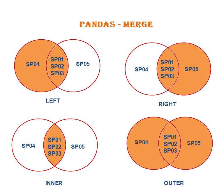
When doing a merge, you can do "left", "right", "inner", and "outer". See the figure below. Imagine SP01-SP04 are dates. For our case, the r_f_4wk table starts in July, 2001. However, the stock_return starts in February, 2000. So when we do a "left" merge, we will have the original rows in stock_return plus whatever wa can match in r_f_4wk, and the rest of the rows that cannot be matched with any row from r_f_4wk will be set as missing.

# I will create a table (main_data) which will have all the stock returns + the columns I want from r_f_4wk
# In my case, I only want the column "r_f_eff", so I specify it as: r_f_4wk['r_f_eff']

main_data = stock_return.merge(r_f_4wk['r_f_eff'], how= 'left', on='Date')

# Here I am renaming my new column that I added to something readable 

main_data.rename(columns = {"r_f_eff": "Risk-free"}, inplace= True)


main_data.head(n=20)

	AMZN	BA	CVX	DIS	GOLD	HSY	INTC	K	KO	M	MMM	MSFT	NVDA	^W5000	Risk-free
Date
2000-02-29	0.066796	-0.169944	-0.106876	-0.063683	-0.003817	0.033823	0.142135	0.043814	-0.153428	-0.118618	-0.058077	-0.086847	0.726798	0.021192	NaN
2000-03-31	-0.027223	0.027196	0.248126	0.213235	-0.038314	0.115744	0.167939	0.028578	-0.034704	0.151618	0.010757	0.188813	0.320071	0.058114	NaN
2000-04-30	-0.176306	0.049587	-0.079108	0.057576	0.071713	-0.066666	-0.038845	-0.058253	0.010433	-0.195267	-0.021877	-0.343529	0.054929	-0.052775	NaN
2000-05-31	-0.124575	-0.015748	0.085903	-0.032951	0.078067	0.140110	-0.016757	0.252578	0.129629	0.132353	-0.010102	-0.103047	0.280503	-0.036091	NaN
2000-06-30	-0.248383	0.074325	-0.076026	-0.080000	0.008687	-0.060264	0.072446	-0.012356	0.076113	-0.123376	-0.025795	0.278721	0.113913	0.043327	NaN
2000-07-31	-0.170396	0.167414	-0.068718	-0.006441	-0.122958	-0.046392	-0.001403	-0.128152	0.070924	-0.287037	0.085090	-0.127343	-0.056048	-0.021162	NaN
2000-08-31	0.377593	0.098912	0.070030	0.010130	0.000981	-0.077026	0.121723	-0.106024	-0.141437	0.148702	0.032790	0.000000	0.322916	0.071246	NaN
2000-09-30	-0.073795	0.205923	0.016603	-0.018050	-0.044075	0.275952	-0.444732	0.053983	0.047195	-0.054834	-0.014390	-0.136079	0.031497	-0.046688	NaN
2000-10-31	-0.047154	0.051357	-0.036657	-0.063726	-0.122951	0.003464	0.082706	0.049095	0.098729	0.246411	0.060356	0.141969	-0.241031	-0.021938	NaN
2000-11-30	-0.325939	0.018433	-0.003044	-0.191972	0.121495	0.164557	-0.154166	-0.029557	0.037267	-0.063339	0.033636	-0.166969	-0.348252	-0.100524	NaN
2000-12-31	-0.369620	-0.042287	0.039316	0.000000	0.100101	0.022559	-0.209843	0.076168	-0.024202	0.147541	0.213949	-0.244009	-0.190975	0.016670	NaN
2001-01-31	0.112450	-0.113636	-0.013708	0.059518	-0.055555	-0.075728	0.230770	-0.001905	-0.048205	0.273143	-0.081742	0.407781	0.575589	0.037408	NaN
2001-02-28	-0.411552	0.063248	0.028578	0.016420	0.047188	0.077142	-0.228041	0.014886	-0.085690	0.085054	0.018978	-0.033777	-0.134382	-0.095482	NaN
2001-03-31	0.004172	-0.101649	0.032789	-0.075929	-0.117901	0.086283	-0.078258	0.026145	-0.148407	-0.140641	-0.073610	-0.073093	0.452797	-0.068221	NaN
2001-04-30	0.542522	0.109316	0.099772	0.057692	0.150454	-0.128534	0.174727	-0.056603	0.026496	0.034416	0.145428	0.238857	0.283078	0.081404	NaN
2001-05-31	0.057668	0.017638	-0.005282	0.045289	0.003650	0.003807	-0.126173	0.047843	0.026196	0.042345	-0.003613	0.021107	0.027732	0.008492	NaN
2001-06-30	-0.152187	-0.113585	-0.051319	-0.086338	-0.076034	0.022515	0.083611	0.095974	-0.050633	-0.051339	-0.032869	0.055219	0.083401	-0.017491	NaN
2001-07-31	-0.117314	0.052698	0.009834	-0.087920	-0.017162	-0.021877	0.019145	0.036896	-0.004988	-0.091765	-0.019457	-0.093288	-0.127763	-0.017414	0.003009
2001-08-31	-0.284227	-0.125235	-0.007003	-0.034915	0.075890	0.068258	-0.062059	0.063851	0.091255	-0.059326	-0.069539	-0.138087	0.047095	-0.061865	0.002902
2001-09-30	-0.332215	-0.343707	-0.059488	-0.267794	0.083022	0.018718	-0.268500	-0.054849	-0.037395	-0.223354	-0.049462	-0.103068	-0.351433	-0.090550	0.002200

# Let's change the format of the Date index to not include the day
# Only year (Y) and month (m)
# I can use a function called strftime, it changes a date to any format I like
# I want it to be year with 4 digits then month, and (-) between the year and month:

main_data.index = main_data.index.strftime('%Y-%m')

main_data.head()

	AMZN	BA	CVX	DIS	GOLD	HSY	INTC	K	KO	M	MMM	MSFT	NVDA	^W5000	Risk-free
Date
2000-02	0.066796	-0.169944	-0.106876	-0.063683	-0.003817	0.033823	0.142135	0.043814	-0.153428	-0.118618	-0.058077	-0.086847	0.726798	0.021192	NaN
2000-03	-0.027223	0.027196	0.248126	0.213235	-0.038314	0.115744	0.167939	0.028578	-0.034704	0.151618	0.010757	0.188813	0.320071	0.058114	NaN
2000-04	-0.176306	0.049587	-0.079108	0.057576	0.071713	-0.066666	-0.038845	-0.058253	0.010433	-0.195267	-0.021877	-0.343529	0.054929	-0.052775	NaN
2000-05	-0.124575	-0.015748	0.085903	-0.032951	0.078067	0.140110	-0.016757	0.252578	0.129629	0.132353	-0.010102	-0.103047	0.280503	-0.036091	NaN
2000-06	-0.248383	0.074325	-0.076026	-0.080000	0.008687	-0.060264	0.072446	-0.012356	0.076113	-0.123376	-0.025795	0.278721	0.113913	0.043327	NaN

---

Returns over time

Let us look at how the historical stock returns were behaving over the time of our analysis:

# I will use a style called "bmh" to make a plot for the monthly returns over time
with plt.style.context('bmh'):
    main_data[["HSY", "NVDA", "^W5000", "Risk-free"]].plot(title = 'Monthly Returns',
                                                # adding a label for the X axis
                                                 xlabel = "Years",
                                                 # adding a label for the Y axis
                                                 ylabel = "Returns",
                                                 # Show grids
                                                 grid=True,
                                                 # specify the size of the chart
                                                 figsize=(10,7),
                                                 # specify the width of the line
                                                 lw=1.5)



plt.show()

Notice some stocks have a lot of jumps; meaning that in some months they have very high returns or very low returns. On the opposite side is the Risk-free return. It is basically stable over time and has not changed a lot.

---

Descriptive Statistics

Lets have a deeper look at the monthly stock returns.

# Descriptive Stats
main_data.describe()

	AMZN	BA	CVX	DIS	GOLD	HSY	INTC	K	KO	M	MMM	MSFT	NVDA	^W5000	Risk-free
count	287.000000	287.000000	287.000000	287.000000	287.000000	287.000000	287.000000	287.000000	287.000000	287.000000	287.000000	287.000000	287.000000	287.000000	270.000000
mean	0.021791	0.012425	0.009857	0.006993	0.008019	0.011105	0.006905	0.006957	0.006149	0.010586	0.007103	0.012066	0.037451	0.005589	0.001137
std	0.129926	0.095598	0.069003	0.076331	0.114357	0.057571	0.097305	0.049571	0.050764	0.129830	0.060703	0.081098	0.174041	0.045973	0.001328
min	-0.411552	-0.454664	-0.214625	-0.267794	-0.381056	-0.177236	-0.444732	-0.138635	-0.172743	-0.628874	-0.157036	-0.343529	-0.486549	-0.177406	0.000000
25%	-0.048718	-0.042805	-0.029320	-0.034121	-0.065294	-0.025150	-0.047195	-0.021066	-0.024000	-0.061762	-0.028618	-0.037006	-0.054362	-0.021149	0.000059
50%	0.021677	0.015899	0.008623	0.005748	0.007592	0.008661	0.007671	0.009467	0.008547	0.011221	0.010560	0.017244	0.030835	0.011240	0.000737
75%	0.087617	0.070993	0.046279	0.050940	0.072783	0.044363	0.062263	0.035843	0.038312	0.077279	0.039402	0.055028	0.122157	0.034368	0.001752
max	0.621776	0.459312	0.269666	0.248734	0.426362	0.275952	0.337428	0.252578	0.141928	0.644123	0.213949	0.407781	0.826231	0.133806	0.004398

We can see NVDA has the highest average monthly return at 3.75%. And the Market index ^W5000 has the lowest average monthly return at 0.56%.

Notice also that NVDA has the highest standard deviation $\sigma$, meaning the highest risk among our list of stocks.

Now with 14 securities + the T-bill, it is quite difficult to know which one would be a good stock to invest in. Because some have high returns but also are accompanied with high risk (such as NVDA), and some have a lot lower average monthly return but also a lower risk as well (such as the market index).

One approach to evaluate these stocks to a standard is to measure the Sharpe Ratio:

$$Sharpe = \frac{E(R_{i}) - R_{f}}{\sigma_{i}}$$

The Sharpe ratio basically measures what is the return you receive for each unit of risk you are taking. An investment that gives you a higher Sharpe ratio (Meaning the highest return per unit of risk) is an investment that gives you a better deal overall.

# Sharpe ratio for DIS
sharpe = (main_data['DIS'].mean() - main_data['Risk-free'].mean())/(main_data['DIS'].std())

print(sharpe)

0.07671412759994857

# Sharpe ratio for BA

sharpe = (main_data['BA'].mean() - main_data['Risk-free'].mean())/(main_data['BA'].std())

print(sharpe)

0.11807858561241205

# Let us go through all the stocks and print their sharpe ratios, 
# but instead of writing the code above 14 times, I will make a (loop)

# A loop means to go through each column (except the last one because it 
# is the return on T-bill "risk-free return") and apply the same set of commands:

# for each column (x) in the table main_data
for x in main_data.columns:
    # if the column is not named "Risk Free" then do the following (not equal is "!=")
    if x != "Risk-free":
        # Measure the sharpe ratio for the column x
        sharpe = (main_data[x].mean() - main_data['Risk-free'].mean())/(main_data[x].std())
        # Print the word "Sharpe Ratio for", then print the column name (x), then the variable sharpe 
        print("Sharpe Ratio for " + x + ":", sharpe)

Sharpe Ratio for AMZN: 0.1589637365765653
Sharpe Ratio for BA: 0.11807858561241205
Sharpe Ratio for CVX: 0.12637140972188973
Sharpe Ratio for DIS: 0.07671412759994857
Sharpe Ratio for GOLD: 0.06017584469299582
Sharpe Ratio for HSY: 0.17314587189384326
Sharpe Ratio for INTC: 0.0592721326989779
Sharpe Ratio for K: 0.11740215408141376
Sharpe Ratio for KO: 0.09872493337254798
Sharpe Ratio for M: 0.07278042594214636
Sharpe Ratio for MMM: 0.0982770773683789
Sharpe Ratio for MSFT: 0.13475647952193534
Sharpe Ratio for NVDA: 0.20865013582209396
Sharpe Ratio for ^W5000: 0.09684057148910538

Let me return to the descriptive statistics table. I would like first to save the table so I can manipulate it by adding columns or rows:

# First, save the results in a dataframe table
desc = main_data.describe()

# Second, transpose the table (i.e., flip it by making the rows column and columns rows)
# save it using the same name (basically overwriting the DataFrame)
desc = desc.transpose()

desc

	count	mean	std	min	25%	50%	75%	max
AMZN	287.0	0.021791	0.129926	-0.411552	-0.048718	0.021677	0.087617	0.621776
BA	287.0	0.012425	0.095598	-0.454664	-0.042805	0.015899	0.070993	0.459312
CVX	287.0	0.009857	0.069003	-0.214625	-0.029320	0.008623	0.046279	0.269666
DIS	287.0	0.006993	0.076331	-0.267794	-0.034121	0.005748	0.050940	0.248734
GOLD	287.0	0.008019	0.114357	-0.381056	-0.065294	0.007592	0.072783	0.426362
HSY	287.0	0.011105	0.057571	-0.177236	-0.025150	0.008661	0.044363	0.275952
INTC	287.0	0.006905	0.097305	-0.444732	-0.047195	0.007671	0.062263	0.337428
K	287.0	0.006957	0.049571	-0.138635	-0.021066	0.009467	0.035843	0.252578
KO	287.0	0.006149	0.050764	-0.172743	-0.024000	0.008547	0.038312	0.141928
M	287.0	0.010586	0.129830	-0.628874	-0.061762	0.011221	0.077279	0.644123
MMM	287.0	0.007103	0.060703	-0.157036	-0.028618	0.010560	0.039402	0.213949
MSFT	287.0	0.012066	0.081098	-0.343529	-0.037006	0.017244	0.055028	0.407781
NVDA	287.0	0.037451	0.174041	-0.486549	-0.054362	0.030835	0.122157	0.826231
^W5000	287.0	0.005589	0.045973	-0.177406	-0.021149	0.011240	0.034368	0.133806
Risk-free	270.0	0.001137	0.001328	0.000000	0.000059	0.000737	0.001752	0.004398

# I will use the same risk free rate assumption as my Excel example
risk_free = 0.004
# Add a column to this newly created table and call it "sharpe"
desc['sharpe'] = (desc["mean"] - risk_free) / desc["std"]

# I would like to drop the last row; which is indexed as "Risk Free"
desc.drop(index = 'Risk-free', inplace= True)

desc

	count	mean	std	min	25%	50%	75%	max	sharpe
AMZN	287.0	0.021791	0.129926	-0.411552	-0.048718	0.021677	0.087617	0.621776	0.136929
BA	287.0	0.012425	0.095598	-0.454664	-0.042805	0.015899	0.070993	0.459312	0.088132
CVX	287.0	0.009857	0.069003	-0.214625	-0.029320	0.008623	0.046279	0.269666	0.084883
DIS	287.0	0.006993	0.076331	-0.267794	-0.034121	0.005748	0.050940	0.248734	0.039208
GOLD	287.0	0.008019	0.114357	-0.381056	-0.065294	0.007592	0.072783	0.426362	0.035141
HSY	287.0	0.011105	0.057571	-0.177236	-0.025150	0.008661	0.044363	0.275952	0.123418
INTC	287.0	0.006905	0.097305	-0.444732	-0.047195	0.007671	0.062263	0.337428	0.029851
K	287.0	0.006957	0.049571	-0.138635	-0.021066	0.009467	0.035843	0.252578	0.059650
KO	287.0	0.006149	0.050764	-0.172743	-0.024000	0.008547	0.038312	0.141928	0.042329
M	287.0	0.010586	0.129830	-0.628874	-0.061762	0.011221	0.077279	0.644123	0.050730
MMM	287.0	0.007103	0.060703	-0.157036	-0.028618	0.010560	0.039402	0.213949	0.051115
MSFT	287.0	0.012066	0.081098	-0.343529	-0.037006	0.017244	0.055028	0.407781	0.099455
NVDA	287.0	0.037451	0.174041	-0.486549	-0.054362	0.030835	0.122157	0.826231	0.192201
^W5000	287.0	0.005589	0.045973	-0.177406	-0.021149	0.011240	0.034368	0.133806	0.034567

# Example to show how useful this table:



# Finding the stock with the highest sharpe ratio:
print('The ticker with the highest Sharpe ratio: \n', desc['sharpe'].idxmax(), '\t', desc['sharpe'].max())

# Finding the stock with the highest average return:
print('The ticker with the highest expected return: \n', desc['mean'].idxmax(),'\t', desc['mean'].max())

# Finding the stock with the highest average return:
print('The ticker with the lowest expected return: \n', desc['mean'].idxmin(),'\t', desc['mean'].min())


# Finding the stock with the highest risk:
print('The ticker with the highest estimated risk: \n', desc['std'].idxmax(), '\t', desc['std'].max())

# Finding the stock with the lowest risk:
print('The ticker with the lowest estimated risk: \n', desc['std'].idxmin(), '\t', desc['std'].min())

The ticker with the highest Sharpe ratio: 
 NVDA 	 0.19220080202651832
The ticker with the highest expected return: 
 NVDA 	 0.03745089165405311
The ticker with the lowest expected return: 
 ^W5000 	 0.005589151215983193
The ticker with the highest estimated risk: 
 NVDA 	 0.17404137392432853
The ticker with the lowest estimated risk: 
 ^W5000 	 0.04597263111366421

As can be seen from the results, the highest Sharpe ratio is found in NVDA. Which means that it is a good stock to invest in.

Notice also that the security with the lowest expected return is also the same security with the lowest estimated risk (^W5000). We can conclude that generally speaking the market offers different securities to match every investor's taste and yet it is competitive and efficient. You want high risk you generally are rewarded with higher expected returns, you want lower risk you will be rewarded with lower expected returns.

QUESTION: Can I have a higher Sharpe ratio than the ones offered by these 14 tickers? Let me examine this question by creating a portfolio that invests say 30% in HSY and 70% in NVDA:

---

Measuring Portfolio Returns

The return for any portfolio consisting of $n$ stocks: $$R_{p} = \sum^{n}_{i=1} w_{i}\times R_{i}$$

where $w$ is the weight for any stock $i$.

Also remember that weights have to sum up to 1: $$\sum^{n}_{i=1} w_{i} = 1$$

main_data['Port_1'] = (0.3 * main_data['HSY']) + (0.7 * main_data['NVDA'])

main_data[['Port_1']].describe()

	Port_1
count	287.000000
mean	0.029547
std	0.122414
min	-0.358341
25%	-0.038771
50%	0.024024
75%	0.091934
max	0.605258

Note Port_1 has an estimated return of 2.95% and a risk of 12.24%.

I would like to see the histogram of returns for this portfolio, and compare it with its components (HSY & NVDA). The steps for creating a histogram is similar to the steps for creating a plot:

# We will use a theme called "classic" 
with plt.style.context('classic'):
    # Note I can customize the histogram by choosing the number of bins and the color of the edges
    hist = main_data['Port_1'].plot.hist(bins = 15, ec="black")
    hist.set_xlabel("Monthly returns")
    hist.set_ylabel("Count")
    hist.set_title("Portfolio 1 Monthly Returns Histogram")

#plt.savefig('Port_1_histogram.png', dpi = 400)
plt.show()

with plt.style.context('ggplot'):
    hist = main_data['HSY'].plot.hist(bins = 15, ec="black")
    hist.set_xlabel("Monthly returns")
    hist.set_ylabel("Count")
    hist.set_title("HSY Monthly Returns Histogram")

#plt.savefig('HSY_histogram.png', dpi = 400)
plt.show()

with plt.style.context('ggplot'):
    hist = main_data['NVDA'].plot.hist(bins = 15, ec="black")
    hist.set_xlabel("Monthly returns")
    hist.set_ylabel("Count")
    hist.set_title("NVDA Monthly Returns Histogram")

#plt.savefig('NVDA_histogram.png', dpi = 400)
plt.show()

# I will plot to histogram in one picture to compare the distribution of returns


with plt.style.context('ggplot'):
    # first histogram is the NVDA stock, I choose the color blue for it
    hist = main_data['NVDA'].plot.hist(color = 'blue', bins = 20, ec="black")
    # first histogram is the Port_1, I choose the color red for it. 


    # Notice I also made this histogram's transparency set to 70%. That way I can see any information behind the bars 
    hist = main_data['Port_1'].plot.hist(color = 'red', bins = 20, ec="black", alpha = 0.7)


    hist.set_xlabel("Monthly returns")
    hist.set_ylabel("Count")
    hist.set_title("Portfolio 1 vs. NVDA Monthly Returns Histogram")

    # I asked to show the definition for each color 
    hist.legend()

#plt.savefig('Port_1_histogram.png', dpi = 400)
plt.show()

From the graph above, I can conclude that the distribution of returns for Port_1 is closer to the mean (centered in the middle) when compared to the returns of NVDA. This means a lower risk!

# Let us examine its Sharpe ratio
sharpe = (main_data['Port_1'].mean() - risk_free)/(main_data['Port_1'].std())
print(sharpe)

0.20869598932150724

As can be seen from this result, I can have a higher Sharpe ratio than HSY or NVDA alone if I made a portfolio investing 30% in HSY and 70% in NVDA; 0.21 vs. 0.19 or 0.12.

Because of diversification, I can create an investment with lower risk (meaning lower $\sigma$), making the denominator in the Sharpe ratio formula smaller, which inturn makes the Sharpe ratio larger.

But why should I stop with two stocks? Maybe I should try to include more stocks in the portfolio, and also try different weights instead of 30% and 70%.

However, with my current setting, this would require me to make a column each time I change weights or add additional stocks. It basically becomes a guessing game...

Is there a way to ask the computer to try different weights on the 14 tickers until it finds a portfolio that has the highest Sharpe ratio? Yes there is a way. But before I jump into it, I need to review how portfolio risk is actually estimated, and also *examine how stock returns behave when they are compared with each other.*

---

Calculating Portfolio Risk (Markowitz Method)

The risk of any portfolio can be measured as the standard deviation of the portfolio return $\sigma_{p}$. However, if the portfolio consists of 2 securities, the standard deviation of the portfolio will not be simply the weighted average of the standard deviation for the two securities.

We need to consider the covariance/correlation between the securities. The covariance reflects the co-movement of returns between the two stocks. Unless the two assets are perfectly positively correlated, the covariance will reduce the overall risk of the portfolio. $$ \rho_{i,j} \,\, or \,\, Corr(R_{i}, R_{j}) = \frac{Cov(R_{i}, R_{j}) \, or\, \sigma_{i,j}}{\sigma_{i}\sigma_{j}} $$

The Variance for any portfolio consisting of $N$ stocks: $$ \sigma^{2}_{p} = \sum^{N}_{j=1} w_{j} \sum^{N}_{i=1} w_{i}\sigma_{ij} $$

Then the portfolio risk* becomes*: $$ \sigma_{p} = \sqrt{\sigma^{2}_{p}} $$

So for our example of Port_1, we have 2 stocks; stock 1 (HSY), and stock 2 (NVDA). Applying the formula:

$$\sigma^{2}_{Port(1)} = w_{1}w_{1}\sigma_{1,1} + w_{1}w_{2}\sigma_{1,2} + w_{2}w_{2}\sigma_{2,2} + w_{2}w_{1}\sigma_{2,1}$$$$\sigma^{2}_{Port(1)} = [0.3 \times 0.3 \times \sigma_{HSY,HSY}] + [0.3 \times 0.7 \times \sigma_{HSY,NVDA}] + [0.7 \times 0.7 \times \sigma_{NVDA,NVDA}] + [0.7 \times 0.3 \times \sigma_{NVDA,HSY}] $$

Since:

• The covariance of stock 1 with itself is the variance ($\sigma_{1,1} = \sigma^{2}_{1}$)

• According to the correlation equation above: $\sigma_{2,1} = \sigma_{1,2} = \rho_{1,2} \sigma_{1} \sigma_{2}$

The equation becomes: $$ \sigma^{2}_{Port(1)} = w^{2}_{1}\sigma^{2}_{1} + w^{2}_{2}\sigma^{2}_{2} + 2 \times (w_{1}w_{2}\sigma_{1}\sigma_{2} \rho_{1,2}) $$

And Port_1's risk is:

$$ \sigma_{Port(1)} = \sqrt{\sigma^{2}_{Port(1)}} $$

Using Matrices

Now for portfolio 1 the above calculations can be relativity easy to calculate. But when I have 3 stocks, or 10 stocks, measuring a portfolio risk can be a very long and tiring equation. Fortunately, I can use matrices in python to make these calculations fast, easy, and consistent.

If I "translate" the above portfolio variance equation into matrices. It will take the following form:

$$ \sigma^{2}_{p} = \begin{bmatrix} w_{1} & w_{2} & \dots & w_{n}\end{bmatrix} \begin{bmatrix} \sigma^{2}_{1} & \sigma_{1,2} & \dots & \sigma_{1,n} \\ \sigma_{2,1} & \sigma^{2}_{2} & \dots & \sigma_{2,n} \\ \dots & &\ddots & \vdots\\ \sigma_{n,1} & \sigma_{n,2} & \dots & \sigma^{2}_{n}\end{bmatrix} \begin{bmatrix} w_{1} \\ w_{2} \\ \vdots \\ w_{n}\end{bmatrix} $$

Now let me use matrix here to measure the standard deviation of a new portfolio (call it "Portfolio 2") where I invest 20% in Nvidia (NVDA), 30% in Microsoft (MSFT), and 50% in CocaCola (KO):

# I will create a list of portfolio weights
w_list =[0.2, 0.3, 0.5]

# The package (Numpy) will be very helpful here 
# (notice I gave it a nickname "np" at the beginning of this notebook)
# It can deal with matrix multiplication and create random numbers if I want
# put the list of weights in a matrix
w = np.array([w_list])

print(w)

[[0.2 0.3 0.5]]

# Make sure the weights always sum up to 1.
# Here I write a statement that the sum of all the elements in a matrix is equal to 1. 
# The computer will tell me if that statement is true or false
np.sum(w) == 1

True

I need a 3 by 3 matrix of covariance for the stocks I want to make a portfolio from ('NVDA','MSFT','KO'). To do that, I first take a slice of the (main_data) which includes only the stocks I care about now. Then save it using a new name (slice)

slice = main_data[['NVDA', 'MSFT', 'KO']]
# Lets see this DataFrame
slice.head()

	NVDA	MSFT	KO
Date
2000-02	0.726798	-0.086847	-0.153428
2000-03	0.320071	0.188813	-0.034704
2000-04	0.054929	-0.343529	0.010433
2000-05	0.280503	-0.103047	0.129629
2000-06	0.113913	0.278721	0.076113

# The covariance table for the dataset (slice)
covariance = slice.cov()

print(covariance)

          NVDA      MSFT        KO
NVDA  0.030290  0.005527  0.000231
MSFT  0.005527  0.006577  0.001013
KO    0.000231  0.001013  0.002577

# Take the covariance table and put it in a matrix
# I will reuse the same variable name (it will overwrite)
covariance_matrix = np.array(covariance)

covariance_matrix

array([[0.0302904 , 0.00552749, 0.00023095],
       [0.00552749, 0.00657686, 0.00101322],
       [0.00023095, 0.00101322, 0.00257697]])

# Notice I can do all the three steps in one line like this

covariance_matrix = np.array(main_data[['NVDA', 'MSFT', 'KO']].cov())

covariance_matrix

array([[0.0302904 , 0.00552749, 0.00023095],
       [0.00552749, 0.00657686, 0.00101322],
       [0.00023095, 0.00101322, 0.00257697]])

# Now I have matrix 1 and 2, whats left is matrix 3
# matrix 3 is basically the "transpose" of matrix 1
# Let me create it
w_vertical= w.T

print(w_vertical)

[[0.2]
 [0.3]
 [0.5]]

Now I apply the above matrix formula. It will look like this:

$$\sigma^{2}_{p} = \begin{bmatrix} w_{NVDA} & w_{MSFT} & w_{KO}\end{bmatrix} \begin{bmatrix} \sigma^{2}_{NVDA} & \sigma_{NVDA,MSFT} & \sigma_{NVDA,KO} \\ \sigma_{MSFT,NVDA} & \sigma^{2}_{MSFT} & \sigma_{MSFT,KO} \\ \sigma_{KO,NVDA} & \sigma_{KO,MSFT} & \sigma^{2}_{KO}\end{bmatrix} \begin{bmatrix} w_{NVDA} \\ w_{MSFT} \\ w_{KO}\end{bmatrix} $$

# The way matrix multiplication is done in Python is through the use of the function (.dot) in Numpy

# First matrix times the 2nd matrix
first = w.dot(covariance_matrix) 

# The answer is then multiplied by the 3rd matrix
second = first.dot(w_vertical)


# Alternatively, embed the first onto the second
# The code is more efficient that way ;)

port_cov = w.dot(covariance_matrix).dot(w_vertical)


print(port_cov)

[[0.00346123]]

# Take out the answer from the matrix:
port_cov[0,0]

0.0034612305695005154

# Thus, the risk for this portfolio is the square root of the calculated variance:

port2_risk = port_cov[0,0] **0.5

port2_risk

0.05883222390408606

Thus, the risk of Port_2 is about 5.87% and it's return (using the data_main[column name].mean() method) is:

port2_return = (main_data['NVDA'].mean()* 0.2)+(main_data['MSFT'].mean()*0.3)+(main_data['KO'].mean()* 0.5)

port2_return

0.014184255809107784

Measuring the Sharpe Ratio:

port2_sharpe = (port2_return - risk_free)/port2_risk

port2_sharpe

0.17310676247274173

So portfolio 2 is not an improvement over portfolio 1...

---

Exporting Datasets

The pandas package offers its users a way to export their tables and datasets to any type of file. It also offers options to import files into a new dataset. In the following code I will export the dataset I have created earlier (main_data) to an Excel file. The produced Excel file will be located in the same folder where this Jupyter Notebook exists.

main_data.to_excel("returns_cleaned.xlsx")