Getting Things Started
In this document, we will learn how to obtain security historical prices, measure returns, run some descriptive analysis on these returns, and visualize them, all with the help of Python. Such an exercise can help us understand and assess a security's overall risk, downside risk, and wether the distribution of the asset's returns have the characteristics of a normal distribution. This notebook will attempt to break each step, and explain each new line of command. Hopefully, by the end of this notebook you will have a better understanding of how python is valuable for a financial analyst.
Unlike a regular Python file script (that has a file ending with .py), Jupyter Notebook files (.ipynb) allow us to run each collection of commands separately in cells.
Loading Packages
The most important package needed in our task is a package that allows us to download data from Yahoo Finance directly to our computer. This package is called yfinance. By default, the package is not available in either your system or in the Anaconda Distribution Platform, so if you are using this package for the first time on your computer, you need to run the following code (again either in Anaconda or in the terminal): pip install yfinance
The rest of the packages are usually available and should load with no issues.
# This package is used for downloading stock data from Yahoo Finance
# we will import it in our project and give it a nickname (yf)
import yfinance as yf
# This package is important so we can analyze data in an excel like objects
# we will nickname it (pd)
import pandas as pd
# This library will help us use dates and times
import datetime as dt
# The following package allows us to draw figures and charts
import matplotlib as mpl
import matplotlib.pyplot as plt
# Numpy is a package that helps python understand math
import numpy as np
Basic Functions of Python
Python, is an object-oriented programming language. It is unique compared to other programming languages in how easy it is to write and understand the syntax "code". Also, because it is open source, there are so many libraries (i.e., mods) available made by the community. This makes Python highly versatile and popular across many disciplines.
So before I start with the main exercise of this notebook, I would like to introduce some of the basic concepts in Python that I will use a lot throughout this course:
Data Types
There are 4 standard types of data python can understand by default:
Integers, such as 0, 2, -5, 234463
Strings, such as "a", "hello", "1223", "12 Street"
Boolean, which as an indicator True or False
Float, which are numbers with fractions, such as 16.001, -11.356, 0.00004
Then there are data types than can be defined by the user or a package imported in the program. One such example we will use later is a date-time data.
Variables
Variables are names given to data items that may take on one or more values during
a program’s runtime. Variable names have to follow some rules:
- It cannot begin with a number
- It must be a single word
- It must consist of letters and _ symbols only
- Variables in Python which start with _ (underscore) are considered as “Un-useful”
Some examples:
text_variable = 'Salam'
integer_var = 23
float_var = -23.56
bol_var = True
print(text_variable, float_var, bol_var, integer_var)
Salam -23.56 True 23
Comments
Comments are lines of text that are ignored and not read by the program. It can be triggered by the character #.
Arithmetic Operators
+ is the addition operator. You can add two objects as long as they are of the same type. For example, you can add two numbers 1+3 and the result will be 4. Or you can add text objects 'a' + 'b' and the result will be 'ab'. The same rule applies for the subtraction -.
/ is division and * is the multiplication operator, and they are self explanatory for numbers. However, multiplication in text repeats the object n number of times. For example 'a'*3 = 'aaa'.
# Example of addition using integers
x = 3
y = 4
z = x+y

# Example of addition using characters "strings"
t= '1'
r = '34'
w = t+r

print(z)
print(w)
print(z*2)
print(w*2)
7
134
14
134134
Lists in Python
Lists are used to store multiple items in a single variable. You can access elements in a list, and you cen modify a list by adding, removing, and replacing elements. Their usage and some functions are shown below with examples:
my_list = ["Sunday", 12, -24.56, 'Finance']

# Extract the first element and save it in a variable:
# Notice how the first position always starts at 0
extracted_1 = my_list[0]

# If I want the last element in a list, I can call it by specifying the position using negative values
# position "-1" starts from the last element and decreases as you go left: -2, -3,
extracted_last = my_list[-1]

# If I want a slice of this list
extracted_subset = my_list[1:3]

print(extracted_1)
print(extracted_last)
print(extracted_subset)
Sunday
Finance
[12, -24.56]
# Changing value in a list
my_list[3] = 'Marketing'

# Delete values from lists
del my_list[2]

print(my_list)
['Sunday', 12, 'Marketing']
Loops
Loops are one of the most valuable functions in Python. It allows the user to do the same set of commands multiple times, maybe on multiple items as well. This makes your code efficient and clean. Most of the time, loops are used with lists or other objects that are similar to a list. Here is a simple example:
weekdays = ['Sunday', 'Monday', 'Tuesday', 'Wednesday', 'Thursday']

# This is a loop that prints (Today is) and then add the item:
for day in weekdays:
    # Notice here I use the word "day" to reference the item I am using in every loop
    print("Today is " + day)
Today is Sunday
Today is Monday
Today is Tuesday
Today is Wednesday
Today is Thursday
Basic Functions of yfinance
To use any function (module) provided by the yfinance package in a task, we first call it by the nickname we gave it (yf), then use the module name. One important function is (.download). It allows us to obtain historical stock data for any security that is available in Yahoo Finance, and then save it in a pandas DataFrame (a table). If you want to learn more what yfinance can do, you can check its website here.
The function .download requires inputs or additional specifications before you can use it. For example, you want .download to download what? We have to supply this function with the name of the security ticker (or maybe a list of tickers). In the following code, I will download Microsoft stock prices. The ticker for Microsoft is MSFT.
The additional information I have to add in the .download function is related to what type of stock prices I want to download for MSFT. In this example, maybe I want to download monthly stock prices, so I will specify this by writing interval = "1mo". If I happen to want daily prices of MSFT, I will replace the word "1mo" with "1d". The following are valid intervals you can use:
Prices for every minute "1m"
Prices for every 2 minutes "2m"
Prices for every 5 minutes "5m"
Prices for every 15 minutes "15m"
Prices for every 30 minutes "30m"
Prices for every 60 minutes "60m" or "1h"
Prices for every 90 minutes "90m"
Prices for every trading day "1d"
Prices for every 5 trading days "5d"
Prices for every week "1wk"
Prices for every month "1mo"
Prices for every 3 months (a quarter) "3mo"
Another input I need to add is either A) period parameter or B) the (start and end) dates. The period parameter determines how far back I want to download the prices of MSFT stock. For example, I want to download monthly prices for the last year, so I would add period = "1y". The following are valid periods one can use:
All stock data for the last day "1d"
All stock data for the last 5 days "5d"
All stock data for the last month "1mo"
All stock data for the last 3 months "3mo"
All stock data for the last 6 months "6mo"
All stock data for the last year "1y"
All stock data for the last 2 years "2y"
All stock data for the last 5 years "5y"
All stock data for the last 10 years "10y"
All stock data from the beginning of the current year(year-to-date) "ytd"
All stock data "max"
As mentioned earlier, the alternative to period is the 2 parameters start and end, where you specify the dates for the data you want to download. The dates have to be in the format (YYYY-MM-DD). For example the command: (yf.download('MSFT', interval = '1d', start = '2002-02-13', end= '2016-05-25') downloads MSFT daily stock data from February 13th, 2002 until May 25th, 2016.
I will try some examples now:
# Download the last year of monthly stock data for Microsoft.
# Save the dataset in a variable called MSFT_monthly
MSFT_monthly = yf.download('MSFT', period = '1y', interval = "1mo")

# Download the last 3 months of daily stock data for Microsoft.
# Save the dataset in a variable called MSFT_daily
MSFT_daily = yf.download("MSFT", period = '3mo', interval = "1d")

# Download weekly stock data for Microsoft from February 13th, 2002 until May 25th, 2016.
# Save the dataset in a variable called MSFT_weekly
MSFT_weekly = yf.download("MSFT", interval = "1wk", start = '2002-02-13', end = '2016-05-25')
[*********************100%***********************]  1 of 1 completed
[*********************100%***********************]  1 of 1 completed
[*********************100%***********************]  1 of 1 completed
# All three sets of information are saved in pandas DataFrames (datasets)
# We can run commands on each dataset. For example if I want to see
# the first couple of rows, I can call the name of the dataset and use the function ".head(n= number of rows to see)"
MSFT_monthly.head(n=5)


# Notice the data has "Close" price but no "Adj Close"
# That's because yfinance already adjusts the closing price automatically
| Price | Close | High | Low | Open | Volume |
|---|---|---|---|---|---|
| Ticker | MSFT | MSFT | MSFT | MSFT | MSFT |
| Date | |||||
| 2024-03-01 | 417.532288 | 427.555768 | 395.371491 | 408.153876 | 426349600 |
| 2024-04-01 | 386.380096 | 426.116728 | 385.089958 | 420.737812 | 440777700 |
| 2024-05-01 | 411.984650 | 430.314707 | 387.352698 | 389.635260 | 413800800 |
| 2024-06-01 | 444.363647 | 453.530295 | 406.553717 | 413.125452 | 342370400 |
| 2024-07-01 | 415.929108 | 465.639769 | 409.824624 | 446.063708 | 440449200 |
# Similarly, I can see the last couple of rows
# using the function ".tail()"
MSFT_daily.head(n=7)
| Price | Close | High | Low | Open | Volume |
|---|---|---|---|---|---|
| Ticker | MSFT | MSFT | MSFT | MSFT | MSFT |
| Date | |||||
| 2024-12-02 | 430.117584 | 432.133531 | 420.466921 | 420.726411 | 20207200 |
| 2024-12-03 | 430.337128 | 431.604575 | 426.884030 | 428.979833 | 18302000 |
| 2024-12-04 | 436.544678 | 438.790175 | 431.764255 | 432.163448 | 26009400 |
| 2024-12-05 | 441.734253 | 443.770179 | 435.297179 | 437.043677 | 21697800 |
| 2024-12-06 | 442.682373 | 445.207309 | 440.885957 | 441.414895 | 18821000 |
| 2024-12-09 | 445.127441 | 447.432816 | 439.618499 | 441.714302 | 19144400 |
| 2024-12-10 | 442.442841 | 448.720262 | 440.716322 | 443.500747 | 18469500 |
Obtaining Data for Multiple Securities in One Command
By passing a list of tickers instead of one ticker when using the .download function, I can obtain data for multiple tickers using only one command.
# The following is a list of index tickers I would like to analyze
ticker_list = ["^W5000", "AGG", "SPY", "GLD"]


# Instead of using a ticker, now we will pass the list as our input
# Notice here I used "max", meaning go as way back as possible to get all historical prices
main_data = yf.download(ticker_list, period = 'max', interval = "1mo")
[*********************100%***********************] 4 of 4 completed
main_data.head(n=5)
| Price | Close | High | Low | Open | Volume | |||||||||||||||
|---|---|---|---|---|---|---|---|---|---|---|---|---|---|---|---|---|---|---|---|---|
| Ticker | AGG | GLD | SPY | ^W5000 | AGG | GLD | SPY | ^W5000 | AGG | GLD | SPY | ^W5000 | AGG | GLD | SPY | ^W5000 | AGG | GLD | SPY | ^W5000 |
| Date | ||||||||||||||||||||
| 1989-01-01 | NaN | NaN | NaN | 2917.260010 | NaN | NaN | NaN | 2917.260010 | NaN | NaN | NaN | 2718.590088 | NaN | NaN | NaN | 2718.590088 | NaN | NaN | NaN | 0 |
| 1989-02-01 | NaN | NaN | NaN | 2857.860107 | NaN | NaN | NaN | 2947.239990 | NaN | NaN | NaN | 2846.699951 | NaN | NaN | NaN | 2916.889893 | NaN | NaN | NaN | 0 |
| 1989-03-01 | NaN | NaN | NaN | 2915.070068 | NaN | NaN | NaN | 2953.139893 | NaN | NaN | NaN | 2846.639893 | NaN | NaN | NaN | 2846.639893 | NaN | NaN | NaN | 0 |
| 1989-04-01 | NaN | NaN | NaN | 3053.129883 | NaN | NaN | NaN | 3053.129883 | NaN | NaN | NaN | 2920.270020 | NaN | NaN | NaN | 2926.750000 | NaN | NaN | NaN | 0 |
| 1989-05-01 | NaN | NaN | NaN | 3162.610107 | NaN | NaN | NaN | 3168.459961 | NaN | NaN | NaN | 3021.800049 | NaN | NaN | NaN | 3049.719971 | NaN | NaN | NaN | 0 |
Notice in the table main_data, I have a bunch of general columns containing additional columns underneath them; one for each security. For example, the column 'High' contains several columns, each one is the high price for each ticker. This structure is possible in pandas DataFrame, and is referred to as a multi-level index structure. So in my dataset here, the level 0 ones are (Close, High, Low, Open, and Volume), and the level 1 are ('AGG', 'GLD', 'SPY', '^W5000') repeated for every level 0 column.
If I want to extract a specific column from this table and run some analysis on it, I can extract one of the general columns (i.e., level 0), such as 'High' using the structure main_data['High']; like extracting an object from a list but here I am specifying a name instead of a position number. However, because of multi-level columns, if I want a slice of the second level column, say '^W5000' under the 'Open' column, I have to call it using the form main_data[[('Open', '^W5000')]]
general_column = main_data['High']

general_column.head()
| Ticker | AGG | GLD | SPY | ^W5000 |
|---|---|---|---|---|
| Date | ||||
| 1989-01-01 | NaN | NaN | NaN | 2917.260010 |
| 1989-02-01 | NaN | NaN | NaN | 2947.239990 |
| 1989-03-01 | NaN | NaN | NaN | 2953.139893 |
| 1989-04-01 | NaN | NaN | NaN | 3053.129883 |
| 1989-05-01 | NaN | NaN | NaN | 3168.459961 |
specific_column = main_data[[('Open','^W5000')]]
specific_column.head()
| Price | Open |
|---|---|
| Ticker | ^W5000 |
| Date | |
| 1989-01-01 | 2718.590088 |
| 1989-02-01 | 2916.889893 |
| 1989-03-01 | 2846.639893 |
| 1989-04-01 | 2926.750000 |
| 1989-05-01 | 3049.719971 |
# Because we are mostly interested in the "Close" columns for each security

# I can take a slice of the table using the first approach
# and save it in a new object

close_prices = main_data['Close']

close_prices.head()
| Ticker | AGG | GLD | SPY | ^W5000 |
|---|---|---|---|---|
| Date | ||||
| 1989-01-01 | NaN | NaN | NaN | 2917.260010 |
| 1989-02-01 | NaN | NaN | NaN | 2857.860107 |
| 1989-03-01 | NaN | NaN | NaN | 2915.070068 |
| 1989-04-01 | NaN | NaN | NaN | 3053.129883 |
| 1989-05-01 | NaN | NaN | NaN | 3162.610107 |
# Alternatively, I can just drop the columns I do not want and continue to use the original DataFrame "main_data"

main_data.drop(columns = ['High', 'Low', 'Open', 'Volume'], inplace = True)

main_data.head()
| Price | Close | |||
|---|---|---|---|---|
| Ticker | AGG | GLD | SPY | ^W5000 |
| Date | ||||
| 1989-01-01 | NaN | NaN | NaN | 2917.260010 |
| 1989-02-01 | NaN | NaN | NaN | 2857.860107 |
| 1989-03-01 | NaN | NaN | NaN | 2915.070068 |
| 1989-04-01 | NaN | NaN | NaN | 3053.129883 |
| 1989-05-01 | NaN | NaN | NaN | 3162.610107 |
# Now I can use either table
# I will continue to use main_data
# But notice that all ticker columns are under the level 0 column "Close"
# I can drop this level since it is useless to me now

main_data = main_data.droplevel(axis='columns', level = 0)


main_data.head()
| Ticker | AGG | GLD | SPY | ^W5000 |
|---|---|---|---|---|
| Date | ||||
| 1989-01-01 | NaN | NaN | NaN | 2917.260010 |
| 1989-02-01 | NaN | NaN | NaN | 2857.860107 |
| 1989-03-01 | NaN | NaN | NaN | 2915.070068 |
| 1989-04-01 | NaN | NaN | NaN | 3053.129883 |
| 1989-05-01 | NaN | NaN | NaN | 3162.610107 |
Lastly, historical prices for these indices start at different years. In my dataset, I have data on Wilshire 5000 starting from 1989 while historical Gold prices start in 2004. I would like my DataFrame to start at the time where all prices are available, so I would like to drop any row having a missing value:
# This code will call the dataset and modify it by using the function ".dropna"
# drop the index (i.e., row) if there is a missing value and once
# you finish deleting the rows, replace my original dataset "inplace = True"
main_data.dropna(axis = 'index', inplace= True)

main_data.head()
| Ticker | AGG | GLD | SPY | ^W5000 |
|---|---|---|---|---|
| Date | ||||
| 2004-11-01 | 53.781303 | 45.119999 | 80.291916 | 11568.540039 |
| 2004-12-01 | 54.032497 | 43.799999 | 82.565498 | 11971.139648 |
| 2005-01-01 | 54.622414 | 42.220001 | 81.095558 | 11642.570312 |
| 2005-02-01 | 54.256107 | 43.529999 | 82.790787 | 11863.480469 |
| 2005-03-01 | 53.738045 | 42.820000 | 80.958321 | 11638.269531 |
Historical Security Data Using Specific Dates
As mentioned earlier, the start and end parameters allows us to use specific dates for downloading the data. However, instead of writing dates in a form of text: '2002-02-13', one can supply these parameters with a "date variable".
Using a date variable instead of using dates in a text form has many advantages. The most important one is that Python will understand its a date, which means if I want to add or subtract a week from a specific date I can do that easily. Also I can find out what day of the week a specific date is.
To take advantage of this tool, we will use the datetime library, which I gave it a nickname of dt at the beginning of this notebook. Lets see some examples on how to use it:
today = dt.datetime.today()

print(today)
2025-02-23 15:39:49.652079
print(today.date())
2025-02-23
# This is the original date
date = dt.date(year=2002, month=12, day=13)
# Save the weekday of this date
week_day= date.weekday()

# If I want to add 100 days to any date variable
days_added = dt.timedelta(days = 100)

# The new date is basically like a math operation
new_date = date + days_added

# What weekday is this new date?
week_day_new = new_date.weekday()


# I will print all this information on the screen
print('old date:', date, ', day of the week:', week_day)
print('new date:', new_date, ', day of the week:', week_day_new)
old date: 2002-12-13 , day of the week: 4
new date: 2003-03-23 , day of the week: 6
Now lets use the date variable in the yfinance command:
# Download MSFT monthly data from 31st December, 1999 to 31st December, 2023:
start = dt.date(1999,12,31)
end = dt.date(2023,12,31)

MSFT_specific = yf.download('MSFT', start=start, end=end, interval='1mo')

# Lets look at the first rows of this table
MSFT_specific.head()
[*********************100%***********************] 1 of 1 completed
| Price | Close | High | Low | Open | Volume |
|---|---|---|---|---|---|
| Ticker | MSFT | MSFT | MSFT | MSFT | MSFT |
| Date | |||||
| 2000-01-01 | 30.054026 | 36.425633 | 29.132829 | 36.041801 | 1274875200 |
| 2000-02-01 | 27.443966 | 33.777189 | 27.060134 | 30.245937 | 1334487600 |
| 2000-03-01 | 32.625690 | 35.312512 | 27.309622 | 27.520729 | 2028187600 |
| 2000-04-01 | 21.417807 | 29.631804 | 19.959246 | 28.998482 | 2258146600 |
| 2000-05-01 | 19.210779 | 22.722840 | 18.539074 | 22.377391 | 1344430800 |
Visualizing Data
The matplotlib package is useful if we would like to graphically represent our data from the tables. In the following examples, I will make figures and graphs from main_data dataset I have created and modified earlier.
# The following command makes sure the theme of the figures are in their default settings
plt.style.use('default')

# Let us see the evolution of historical price levels for one of our indices
# First, I call the columns in the dataset using double parenthesis [[ ]], then ask to "plot" the information in a graph
# Now the plot is saved by default in "plt"
main_data[['AGG']].plot()

# I can modify the plot by calling 'plt' and setting the new modifications:

# Give the x axis a label name:
plt.xlabel("Date")

# Give the y axis a label name
plt.ylabel("Close Price")

# Make a title for this plot
plt.title("AGG Performance Over Time")

# Save the plot in the folder and name it (first_graph.png)
plt.savefig('first_graph.png', dpi = 400)

# Show the plot we just saved
plt.show()

# Maybe you want to make the figure a bit more beautiful.
# You can make additional customization!

# let us try a black background theme with a red line

# To do it, we need to start the code by writing "with":
# It means apply the following code using the theme (dark_background)
with plt.style.context('dark_background'):

    # <<< notice the code is indented with 4 spaces
    main_data[['SPY']].plot(color='darkred')

    # Let us give the x axis a label name:
    plt.xlabel("Date")

    # Let us give the y axis a label name
    plt.ylabel("Price")

    # Making a title for our graph
    plt.title("SPY Performance Over Time")

# The (with) condition is finished, so we are back writing commands with no spaces

# Save the plot in the folder and name it (black_graph.png)
plt.savefig('black_graph.png', dpi = 400)

plt.show()

# Another fast method is a simple 1 line of code.
# After calling plot, all the customization can be done inside the parenthesis.
# I was able to add a title, a label for the Y axis,
# a label for the X axis, and change the color all inside the function.

one_step_graph = main_data[['GLD']].plot(title="Gold Performance Over Time",
                                    color = 'darkviolet',
                                    ylabel= "Price",
                                    xlabel= 'Year')


plt.show()

# Plotting ticker prices for more than one column
# I just call the dataset without slicing any columns

main_data.plot(title= 'Historical Price Levels of Indices',
                     color = ['red','darkviolet','blue', 'green'],
                     ylabel= "Price",
                     xlabel= 'Year')


plt.show()

The previous plot is not really helpful for understanding which stock performed better during the time period. This is because each index started at a different price level.
To make this plot more informative and better looking, the prices should be adjust, so that they all start at the same level. This is referred to as (Normalizing Security Prices). The price of each security should be adjusted so they all start at a price of 1 at the start of this race: $$Normalized \ Price_{t} = \frac{Price_{t}}{Price_{t=0}}, \quad \quad for \: t \: in \: [0,T]$$
# To extract a value from the dataset, I need to find its location (row number, column number)

# for example, if I want to extract the first row the AGG index:
print(main_data.iloc[0,0])
53.78130340576172
The problem is what if I do not know the position for the column I want?
Well, one way is to use the built-in function .get_loc on the list of column names in my dataset. First, lets call the list of column names of my DataFrame and save it in an object:
column_list = main_data.columns
print(column_list)
Index(['AGG', 'GLD', 'SPY', '^W5000'], dtype='object', name='Ticker')
# Now I will simply apply the function .get_loc to find the position of say 'SPY'
print(column_list.get_loc('SPY'))
2
# Or maybe just use it directly on the command ".columns"
print(main_data.columns.get_loc('SPY'))
2
# So, if I want the first row in the column '^W5000'

answer  = main_data.iloc[0, main_data.columns.get_loc('^W5000')]
print(answer)
11568.5400390625
# Now I will normalize the prices


# create a new column in the DataFrame and name it 'AGG Normal',
# it equals AGG / the first row in AGG

main_data['AGG Normal'] = main_data['AGG'] / main_data.iloc[0, main_data.columns.get_loc('AGG')]

main_data.head()
| Ticker | AGG | GLD | SPY | ^W5000 | AGG Normal |
|---|---|---|---|---|---|
| Date | |||||
| 2004-11-01 | 53.781303 | 45.119999 | 80.291916 | 11568.540039 | 1.000000 |
| 2004-12-01 | 54.032497 | 43.799999 | 82.565498 | 11971.139648 | 1.004671 |
| 2005-01-01 | 54.622414 | 42.220001 | 81.095558 | 11642.570312 | 1.015639 |
| 2005-02-01 | 54.256107 | 43.529999 | 82.790787 | 11863.480469 | 1.008828 |
| 2005-03-01 | 53.738045 | 42.820000 | 80.958321 | 11638.269531 | 0.999196 |
I can do the same steps in the above cell for all tickers. But this will take time and a lot of repetitive code. Alternatively, I can run through all the tickers using a loop!
But before I do that, first let me drop the column I just created:
main_data.drop(columns = 'AGG Normal', inplace=True)
main_data.head()
| Ticker | AGG | GLD | SPY | ^W5000 |
|---|---|---|---|---|
| Date | ||||
| 2004-11-01 | 53.781303 | 45.119999 | 80.291916 | 11568.540039 |
| 2004-12-01 | 54.032497 | 43.799999 | 82.565498 | 11971.139648 |
| 2005-01-01 | 54.622414 | 42.220001 | 81.095558 | 11642.570312 |
| 2005-02-01 | 54.256107 | 43.529999 | 82.790787 | 11863.480469 |
| 2005-03-01 | 53.738045 | 42.820000 | 80.958321 | 11638.269531 |
# Run a loop going through each ticker name (i.e., column)
# In this code I am referring to the column name as x throughout the loop
for x in main_data.columns:
    # Create a new column named x (the original name of the column) + "space" +  the word "Normalized"
    main_data[ x + ' ' + 'Normalized' ] = main_data[x] / main_data.iloc[0, main_data.columns.get_loc(x)]


main_data.head()
| Ticker | AGG | GLD | SPY | ^W5000 | AGG Normalized | GLD Normalized | SPY Normalized | ^W5000 Normalized |
|---|---|---|---|---|---|---|---|---|
| Date | ||||||||
| 2004-11-01 | 53.781303 | 45.119999 | 80.291916 | 11568.540039 | 1.000000 | 1.000000 | 1.000000 | 1.000000 |
| 2004-12-01 | 54.032497 | 43.799999 | 82.565498 | 11971.139648 | 1.004671 | 0.970745 | 1.028316 | 1.034801 |
| 2005-01-01 | 54.622414 | 42.220001 | 81.095558 | 11642.570312 | 1.015639 | 0.935727 | 1.010009 | 1.006399 |
| 2005-02-01 | 54.256107 | 43.529999 | 82.790787 | 11863.480469 | 1.008828 | 0.964761 | 1.031122 | 1.025495 |
| 2005-03-01 | 53.738045 | 42.820000 | 80.958321 | 11638.269531 | 0.999196 | 0.949025 | 1.008300 | 1.006028 |
# lets try the plot now!
# Notice because I am using a subset of the dataset, I should include the columns inside a list
main_data[['AGG Normalized', 'GLD Normalized', 'SPY Normalized', '^W5000 Normalized']].plot(title= 'Historical Performance of Indices',
                     ylabel= "Monthly Normalized Price",
                     xlabel= 'Year')

# I can save this figure as a png file in my folder
plt.savefig('normalized_performance.png', dpi = 400)
plt.show()

This is a full example for a more detailed customization when creating a professional figure:
with plt.style.context('fivethirtyeight'):

    # set the size of the figure (width, height)
    plt.figure(figsize=(10,6))

    # plot the data, each one using a specific label name, color, and line width
    plt.plot(main_data[['AGG Normalized']], label= 'Bond Index', color='blue', linewidth = 2)
    plt.plot(main_data[['GLD Normalized']], label= 'Gold Index', color='purple', linewidth = 2)
    plt.plot(main_data[['SPY Normalized']], label= 'S&P500', color='green', linewidth = 2)
    plt.plot(main_data[['^W5000 Normalized']], label= 'Wilshire 5000', color='red', linewidth = 2)


    # add the label box and give it a name and font size
    plt.legend(title='Index', fontsize = 8)

    # Other customizations add x and y labels and a title

    # Add a Y axis label, make it a size 12, and make the font bold
    plt.ylabel("Monthly Normalized Price Level", fontsize=12, weight = 'bold')
    # Set the Y ticks fontsize to be 9
    plt.yticks(fontsize = 9)
    # Add an X axis label, make it a size 12, and make the font bold
    plt.xlabel('Year', fontsize=12, weight = 'bold')
    # Set the X ticks fontsize to be 9
    plt.xticks(fontsize = 9)
    # Add a figure title
    plt.title('Historical Performance', fontsize=18, weight='bold')


plt.savefig('many_stocks_graph.png', dpi = 400)

plt.show()

It is now clear that the S&P500 performed better than the other 3 indices historically!
Visit the matplotlib website to discover more styles: https://matplotlib.org/stable/gallery/style_sheets/style_sheets_reference.html
Measuring Returns
I need to find a way using pandas to calculate security returns. Specifically, I would like to apply the following formula for each row: $$Return_{t} = \frac{P_{t}-P_{t-1}}{P_{t-1}}$$
Luckily, my dataset has the prices arranged by date in an ascending order (i.e., from oldest to the most recent date). So to apply the above formula, I will use one of the many useful functions provided by pandas, which is .pct_change(). This will calculate the percentage change of the value of each row from its previous value.
# First thing, I do not need the normalized prices anymore
# so I will drop them using a loop

for column in main_data.columns:
    # This is a condition statement:
    if 'Normalized' in column:
        # If the column name has the word "Normalized", then apply the following
        main_data.drop(columns=column, inplace=True)


main_data.head()
| Ticker | AGG | GLD | SPY | ^W5000 |
|---|---|---|---|---|
| Date | ||||
| 2004-11-01 | 53.781303 | 45.119999 | 80.291916 | 11568.540039 |
| 2004-12-01 | 54.032497 | 43.799999 | 82.565498 | 11971.139648 |
| 2005-01-01 | 54.622414 | 42.220001 | 81.095558 | 11642.570312 |
| 2005-02-01 | 54.256107 | 43.529999 | 82.790787 | 11863.480469 |
| 2005-03-01 | 53.738045 | 42.820000 | 80.958321 | 11638.269531 |
# Create a new table (index_returns) that takes the percentage changes of each row in the "main_data" table
index_returns = main_data.pct_change()

index_returns.head()
| Ticker | AGG | GLD | SPY | ^W5000 |
|---|---|---|---|---|
| Date | ||||
| 2004-11-01 | NaN | NaN | NaN | NaN |
| 2004-12-01 | 0.004671 | -0.029255 | 0.028316 | 0.034801 |
| 2005-01-01 | 0.010918 | -0.036073 | -0.017803 | -0.027447 |
| 2005-02-01 | -0.006706 | 0.031028 | 0.020904 | 0.018974 |
| 2005-03-01 | -0.009548 | -0.016311 | -0.022134 | -0.018984 |
# drop the missing values (i.e., the first row)
index_returns.dropna(axis='index', inplace= True)

index_returns.head()
| Ticker | AGG | GLD | SPY | ^W5000 |
|---|---|---|---|---|
| Date | ||||
| 2004-12-01 | 0.004671 | -0.029255 | 0.028316 | 0.034801 |
| 2005-01-01 | 0.010918 | -0.036073 | -0.017803 | -0.027447 |
| 2005-02-01 | -0.006706 | 0.031028 | 0.020904 | 0.018974 |
| 2005-03-01 | -0.009548 | -0.016311 | -0.022134 | -0.018984 |
| 2005-04-01 | 0.016626 | 0.012377 | -0.014881 | -0.023607 |
Now I would like to examine the historical return distribution for AGG. More specifically, I want to examine whether monthly returns for AGG follow a normal distribution.
Do to so, I am going to create a plot object for the column "AGG" located in the "index_returns" DataFrame. The plot will be of kind .hist(). Inside this function, I can add specifications for my plot to customize it, such as the number of binds, the color of the bars, and so on...
# Note here that I will create an
# object "our_hist" which will contain the plot

our_hist = index_returns[['AGG']].plot.hist(bins = 25,
                                            color = "maroon",
                                            ec='black')

# Adding labels to the X and Y axes,
# and a title to the figure we created
our_hist.set_xlabel("Monthly returns")
our_hist.set_ylabel("Count")
our_hist.set_title("AGG Monthly Returns Frequency")

plt.savefig('first_histogram.png', dpi = 400)
# Let's see how it looks like!
plt.show()

# This is for the S&P500
# Same as before, but this time
# using an alternative theme and
# other types of customization

# We will use a theme called "classic"
with plt.style.context('classic'):
    hist = index_returns[['SPY']].plot.hist(bins = 25, alpha=0.9)
    hist.set_xlabel("Monthly returns")
    hist.set_ylabel("Count")
    hist.set_title("S&P500 Monthly Returns Frequency", fontsize = 15)
plt.show()

with plt.style.context('ggplot'):
    plt.plot.hist()
    hist = index_returns[['AGG', '^W5000']].plot.hist(bins = 20,
                                                      alpha=0.75,
                                                      color = ['darkblue', 'maroon'])
    hist.set_xlabel("Monthly returns")
    hist.set_ylabel("Count")
    hist.set_title("Monthly Returns Frequency", fontsize = 15)
plt.show()

# In this example, I am creating 2 separate histograms
# one top of each other in one plt figure

# Note in the customization here, I can specify the degree of transparency
# for each plot using the key: "alpha"; I set it to 80% so I can
# see the distribution for W5000 behind AGG
# Also I set the color and number of binds for each index
with plt.style.context('ggplot'):

    # set the size of the figure (width, height)
    plt.figure(figsize=(10,6))

    # Plot the histograms
    plt.hist(index_returns[['^W5000']], label = 'Wilshire 5000 Index', color = 'maroon', alpha = 0.85, bins = 25)
    plt.hist(index_returns[['AGG']], label = 'Bond Index', color = 'darkblue', alpha = 1, bins = 25)


    # add the label box and give it a name, font size, and a location in the figure
    plt.legend(title='Index', fontsize = 10, loc= 'upper left')

    # Other customizations add x and y labels and a title

    # Add a Y axis label, make it a size 12, and make the font bold
    plt.ylabel("Count", fontsize=12, weight = 'bold')
    # Set the Y ticks fontsize to be 9
    plt.yticks(fontsize = 9)
    # Add an X axis label, make it a size 12, and make the font bold
    plt.xlabel('Monthly Returns', fontsize=12, weight = 'bold')
    # Set the X ticks fontsize to be 9
    plt.xticks(fontsize = 9)
    # Add a figure title
    plt.title('Monthly Return Frequency', fontsize=18, weight='bold')


plt.savefig('two_hist.png', dpi = 400)

plt.show()

Descriptive Statistics and Basic Analysis of Excess Returns
Although the above graphs are useful for having a general idea on the return distribution, they are not that informative. First, they are raw returns, and such returns have occurred while the risk-free rate is changing from one month to another. If I plan to use historical returns to help me predict future returns, I would like examine the excess return probability distribution for each security. In the following section, I will estimate simple descriptive statistics; mean, median, standard deviation (i.e., risk), as well as alternative measures of risk, such as VaR, estimated shortfall, and downside risk on excess returns. I will then rank these alternative investment options (S&P500, Corporate Bonds, Wilshire 5000, and Gold) using both the Sharpe ratio and the Sorinto ratio.
So, the first step is to measure the excess return for each period:
$$Excess \: Return_{t} = R_{t} - R_{f}$$
This means I need to obtain data on historical T-bill prices so I can measure the historical risk-free rate ($R_{f}$). T-bill monthly prices are obtained from the Federal Reserve Bank of St. Louis (FRED). The ID used by FRED for the 4-week-maturity treasury bill is TB4WK. If I am working with annual or daily security returns for example, I probably will need to download something different from FRED. Because the risk-free rate I need to measure must match the investment horizon I am analyzing. (In my case it is monthly)
Recall the U.S. Federal government sells T-bill securities with different maturities; 4, 13, 26, and 52 weeks. Ideally, I would like to measure the return on a T-bill investment that has a maturity matching my investment horizon (Again, for my analysis its 1 month). So for example if I am examining the return of AMZN during the month of April 2016, I would like to compare the security's performance with a T-bill security that was issued by the U.S. government at the beginning of April 2016 and has a maturity of 1 month.
But what if there are no T-bills sold at that specific day, or I do not have this information, or the government does not sell a T-bill matching my investment horizon? Say if my investment horizon is 1 week, what can I do?
Well, to answer this question, remember that T-bills are money market instruments, which means they are financial assets with high liquidity sold and bought in the market on a daily basis. Thus, one can find the approximate return on a T-bill investment of 1 week by looking at the price of a T-bill today then checking its price after 1 week. The holding period return (HPR) for this investment can represent the 1-week risk-free rate: $$R_{f, t} = \frac{P_{1} - P_{0}}{P_{0}}$$
Because T-bills have no risk, we know for certainty that at maturity the investor receives face value. If a 4-week T-bill was issued and sold today for $\$950$, this means the security will pay the holder $\$1,000$ in 4 weeks ($\$50$ profit in 4 weeks). If the investor sells this T-bill after 3 weeks from today, and assuming interest rates on new T-bills have not changed, then logically speaking (and ignoring compounding for a moment) the seller should be entitled for only 3 weeks worth of profits. That is 3/4 of the $\$50$ which is $\$37.50$. Anyone buying this T-bill and holds it for an additional week should receive 1/4 of the $\$50$ ($\$12.50$). Thus, a buyer should be willing to pay ($\$1000 - \$12.50 = \$987.5$) and would receive the face value after one week with certainty.
To put it another way, if a 4-week T-bill has a return of 4%, then holding this security for 3 weeks should provide the investor (3/4 of the 4% = 3%) return. More importantly, because of market efficiency, any two short-term T-bills having different maturities should at least give an investor the same return when buying and holding them for the same period; because they are issued by the same borrower: the U.S. government.
Calculating $R_{f}$ from T-bill quotes
Remember, The quotes we see on T-bills are annualized using the bank-discount method, which has two main flaws: A) Assumes the year has 360 days, and B) Computes the yield as a fraction of face value instead of the current price. Thus, to find the actual risk-free rate, our first task is to transform the annual yield we get from a bank-discount method to an annual bond-equivalent yield (BD to BEY). This is done by first finding the price of the T-bill:
$$Price = Face \,\, Value \times \left[ 1- (R_{BD} \times \frac{n}{360}) \right] $$
Where $n$ is the number of days until the bill matures. Once we find the price, the Bond-Equivalent Yield (BEY) is basically:
$$R_{BEY} = \frac{Face \,\, Value - Price}{Price} \times \frac{365}{n}$$
Again, $n$ is the number of days until the T-bill I collected information about matures. Think of BEY as another version of the popular APR. Meaning the calculated return is in an annualized form and it ignores any compounding. Now, the simplest way of finding the risk-free return that matches my investment horizon is to divide the BEY by the number of investment periods I have during the year. For example, for monthly analysis, I divide the BEY by 12, for weekly 52, and for daily 365:
$$Monthly \,\, R_{f} = R_{BEY} \times \frac{1}{m} = \frac{R_{BEY}}{12}$$
If I want to be precise and assume compounding, then I apply the following formula for finding the effective risk-free rate:
$$R_{eff.} = \left[ 1 + R_{BEY} \right]^{\frac{1}{m}} -1$$
where $m$ is the divisor (monthly = 12, weekly = 52, yearly = 365 and so on...)
Because my investment horizon is monthly, and there is data on 1-month maturity T-bills. I will simply use the convenient source: (TB4WK) and no conversion is needed once I measure the price. However, to check my conclusions above, I will also download the three-month T-bill data and transform them to monthly using the approach discussed above.
*Note: The 4-week maturity T-bill data offered by FRED starts in mid 2001. If you want to collect monthly rates for older periods, you need to use an alternative source. You can collect T-bill prices for the three-month maturity bills (TB3MS) (starts at the end of 1938) and find the monthly return using the approach I discussed above.
I will import another important package here: (fredapi). This package is made and managed by the Federal Reserve Bank of St. Louis in the United States. Using the package allows the user to download economic data directly from their server. It is basically a portal one can use to obtain any public data provided by the Fed. In order to use this feature, you are required to first open an account at their website, and then request an API Key. From my experience, the API-Key request is approved immediately.
Check this link for more info: https://fred.stlouisfed.org/docs/api/api_key.html
# If it is your first time using fredapi, you need to download it to your anaconda library if you use one.
# You can do it through the anaconda program
# Or alternatively, run the following code here only once on your computer

%pip install fredapi
# If you have installed fredapi, import the package
from fredapi import Fred

# Don't forget to use your api-key after opening account with FRED
# So then you can download any data from their server
fred = Fred(api_key = '44303cd2e2752fc88d6080b1e0d9d1e9')
# the following code obtains the quotes on 4-week maturity t-bills from FRED (reported monthly)
# we will save it in a variable called (r_f_4wk)
r_f_4wk = fred.get_series('TB4WK')

# the following code obtains the discount rates of 3-month maturity t-bills from FRED (reported monthly)
# we will save it in a variable called (r_f_3m)
r_f_3m= fred.get_series('TB3MS')

r_f_4wk.head()
2001-07-01    3.61
2001-08-01    3.48
2001-09-01    2.63
2001-10-01    2.24
2001-11-01    1.96
dtype: float64
# The risk-free rates obtained from FRED are in a (column) form, or we call it "series"
# We need to transform it to a pandas DataFrame
r_f_4wk = r_f_4wk.to_frame()
r_f_3m = r_f_3m.to_frame()

r_f_4wk.head()
| 0 | |
|---|---|
| 2001-07-01 | 3.61 |
| 2001-08-01 | 3.48 |
| 2001-09-01 | 2.63 |
| 2001-10-01 | 2.24 |
| 2001-11-01 | 1.96 |
# I would like to adjust the dates
# column "the dataset's index" so I only
# see dates not date-time
# I will define my new index to equal
# the old index after extracting only the date
r_f_4wk.index = r_f_4wk.index.date

# Rename the index and call it "Date"
r_f_4wk.index.rename('Date', inplace = True)

# the same for the other Dataframe
r_f_3m.index = r_f_3m.index.date
r_f_3m.index.rename('Date', inplace = True)

r_f_4wk.head()
| 0 | |
|---|---|
| Date | |
| 2001-07-01 | 3.61 |
| 2001-08-01 | 3.48 |
| 2001-09-01 | 2.63 |
| 2001-10-01 | 2.24 |
| 2001-11-01 | 1.96 |
# Note the rates are in whole numbers, not fractions. Let's adjust that:
r_f_4wk[0] = r_f_4wk[0]/100
r_f_3m[0] = r_f_3m[0]/100

r_f_4wk.head()
| 0 | |
|---|---|
| Date | |
| 2001-07-01 | 0.0361 |
| 2001-08-01 | 0.0348 |
| 2001-09-01 | 0.0263 |
| 2001-10-01 | 0.0224 |
| 2001-11-01 | 0.0196 |
# Here I am measuring the price using
# the formulas presented above

# Remember the maturity for this T-bill
# is 3-months. which means n = 90
r_f_3m['Price'] = 1000*(1-  (r_f_3m[0] * (90/360))  )
# Then I create a column measuring the BEY
r_f_3m['BEY'] = ((1000 - r_f_3m['Price'])/ r_f_3m['Price']) * (365/90)

# My monthly risk-free rate is dividing the BEY by 12
r_f_3m['r_f_simple'] = r_f_3m['BEY'] / 12

# For more accurate rate, I can assume compounding
# and measure the effective monthly return as well
r_f_3m['r_f_eff'] = (1 + r_f_3m['BEY'])**(1/12) - 1

# lets see the table now
r_f_3m.head()
| 0 | Price | BEY | r_f_simple | r_f_eff | |
|---|---|---|---|---|---|
| Date | |||||
| 1934-01-01 | 0.0072 | 998.200 | 0.007313 | 0.000609 | 0.000607 |
| 1934-02-01 | 0.0062 | 998.450 | 0.006296 | 0.000525 | 0.000523 |
| 1934-03-01 | 0.0024 | 999.400 | 0.002435 | 0.000203 | 0.000203 |
| 1934-04-01 | 0.0015 | 999.625 | 0.001521 | 0.000127 | 0.000127 |
| 1934-05-01 | 0.0016 | 999.600 | 0.001623 | 0.000135 | 0.000135 |
# Similar steps for the 4-week maturity bills:

# The maturity for these bills is weeks, so n = 28
r_f_4wk['Price'] = 1000*(1-  (r_f_4wk[0] * (28/360))  )
# Then I create a column measuring the BEY
r_f_4wk['BEY'] = ((1000 - r_f_4wk['Price'])/ r_f_4wk['Price']) * (365/28)

# My monthly risk-free rate is dividing the BEY by 12
r_f_4wk['r_f_simple'] = r_f_4wk['BEY'] / 12
# For more accuracy, I can assume compounding and use the effective monthly return
r_f_4wk['r_f_eff'] = (1 + r_f_4wk['BEY'])**(1/12) - 1

# lets see the table now
r_f_4wk.head()
| 0 | Price | BEY | r_f_simple | r_f_eff | |
|---|---|---|---|---|---|
| Date | |||||
| 2001-07-01 | 0.0361 | 996.991667 | 0.036712 | 0.003059 | 0.003009 |
| 2001-08-01 | 0.0348 | 997.100000 | 0.035386 | 0.002949 | 0.002902 |
| 2001-09-01 | 0.0263 | 997.808333 | 0.026724 | 0.002227 | 0.002200 |
| 2001-10-01 | 0.0224 | 998.133333 | 0.022754 | 0.001896 | 0.001877 |
| 2001-11-01 | 0.0196 | 998.366667 | 0.019905 | 0.001659 | 0.001644 |
# Let us check if there are differences between
# the 4-week and the 3-month T-bills after
# I adjusted them to my investment horizon

# I will obtain 1 row from the dataset by using a function from pandas
# named (loc). This allows me to specify the index label for the row I want

# Remember my index here are dates, so I want the row matching the date: 1/31/2017
# I will insert the date as a "date object"
the_date = dt.date(2017, 1, 1)

print(r_f_4wk.loc[the_date])

# I would like to compare it with the row from the 3-month T-bills
print(r_f_3m.loc[the_date])
0               0.004900
Price         999.591667
BEY             0.004970
r_f_simple      0.000414
r_f_eff         0.000413
Name: 2017-01-01, dtype: float64
0               0.005100
Price         998.725000
BEY             0.005177
r_f_simple      0.000431
r_f_eff         0.000430
Name: 2017-01-01, dtype: float64
Notice how the difference between the two rates are minimal (The simple monthly $R_{f}$ for the 4-week maturity is 0.0414% and the 3-month maturity is 0.0431%), which means the 3-month is a good approximation for monthly risk-free rate after transforming it! You can check other periods to see whether the difference is big or small...
Merging Two Datasets Using Python
Notice I have two datasets: index_returns which includes monthly index returns and r_f_4wk which includes the monthly risk-free rate. I would like to join them in one table now...
When I have two or more tables and want to combine them, I can use a function in pandas called "merge". This function has so many configurations on how to join DataFrames. But since both of our tables (index_returns, r_f_4wk) have the same index name (Date), the matching process can be done quite easily (I just need to do the same transformation I did for the risk-free table dates; i.e., the date-time rows to be dates only in index_returns).
When doing a merge, you can do "left", "right", "inner", and "outer". See the figure below:
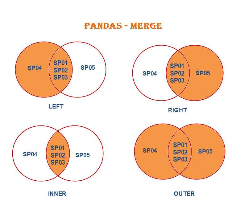
Imagine SP01-SP05 are dates. For our case, the r_f_4wk table starts in July, 2001. However, the index_returns starts in 2004. So when we do an "inner" merge, we will have the matched rows in both tables.
# I am adjusting the dates in the indices return table
index_returns.index = index_returns.index.date

# Renaming the index and call it "Date"
index_returns.index.rename('Date', inplace = True)

index_returns.head()
| Ticker | AGG | GLD | SPY | ^W5000 |
|---|---|---|---|---|
| Date | ||||
| 2004-12-01 | 0.004671 | -0.029255 | 0.028316 | 0.034801 |
| 2005-01-01 | 0.010918 | -0.036073 | -0.017803 | -0.027447 |
| 2005-02-01 | -0.006706 | 0.031028 | 0.020904 | 0.018974 |
| 2005-03-01 | -0.009548 | -0.016311 | -0.022134 | -0.018984 |
| 2005-04-01 | 0.016626 | 0.012377 | -0.014881 | -0.023607 |
# I am creating a table (excess_returns) which will
# have all the indices returns + the columns I want from r_f_4wk

# In my case, I only want the column "r_f_eff",
# so I can specify it as: r_f_4wk['r_f_eff']

excess_returns = index_returns.merge(r_f_4wk['r_f_eff'], how= 'inner', on='Date')

# Renaming my new column that I merged to something readable
excess_returns.rename(columns = {"r_f_eff": "Risk-free"}, inplace= True)

excess_returns.head(n=7)
| AGG | GLD | SPY | ^W5000 | Risk-free | |
|---|---|---|---|---|---|
| Date | |||||
| 2004-12-01 | 0.004671 | -0.029255 | 0.028316 | 0.034801 | 0.001610 |
| 2005-01-01 | 0.010918 | -0.036073 | -0.017803 | -0.027447 | 0.001669 |
| 2005-02-01 | -0.006706 | 0.031028 | 0.020904 | 0.018974 | 0.001943 |
| 2005-03-01 | -0.009548 | -0.016311 | -0.022134 | -0.018984 | 0.002175 |
| 2005-04-01 | 0.016626 | 0.012377 | -0.014881 | -0.023607 | 0.002167 |
| 2005-05-01 | 0.008411 | -0.039216 | 0.032225 | 0.037338 | 0.002167 |
| 2005-06-01 | 0.008642 | 0.042977 | -0.002511 | 0.007544 | 0.002324 |
# Here I am using a loop to
# measure the excess returns
# for each security


for index_name in excess_returns.columns:
    # I am stating a condition, if the
    # column is not named "Risk-free",
    # then proceed and do the following commands...
    if index_name != 'Risk-free':
        # create a column in the table (excess_returns)
        # This column is named "index_name". Basically,
        # means I overwrite the existing column with a new one
        excess_returns[index_name] = excess_returns[index_name] - excess_returns['Risk-free']


excess_returns.head()
| AGG | GLD | SPY | ^W5000 | Risk-free | |
|---|---|---|---|---|---|
| Date | |||||
| 2004-12-01 | 0.003060 | -0.030866 | 0.026706 | 0.033191 | 0.001610 |
| 2005-01-01 | 0.009249 | -0.037742 | -0.019472 | -0.029116 | 0.001669 |
| 2005-02-01 | -0.008649 | 0.029085 | 0.018961 | 0.017031 | 0.001943 |
| 2005-03-01 | -0.011724 | -0.018486 | -0.024309 | -0.021159 | 0.002175 |
| 2005-04-01 | 0.014459 | 0.010210 | -0.017048 | -0.025774 | 0.002167 |
pandas has a command .describe(). It generates a table containing the main statistics for any DataFrame I apply this function on. Specifically, it measures the number of observations, mean, standard deviation, and the minimum, 25th percentile, median, 75th percentile, and max value.
# Here I am generating a descriptive statistics table for our indices
print(excess_returns.describe())
              AGG         GLD         SPY      ^W5000   Risk-free
count  242.000000  242.000000  242.000000  242.000000  242.000000
mean     0.001248    0.007108    0.008035    0.006603    0.001283
std      0.013365    0.048075    0.043707    0.044681    0.001545
min     -0.043659   -0.161616   -0.160574   -0.177626    0.000000
25%     -0.005792   -0.023747   -0.016581   -0.018710    0.000044
50%      0.001838    0.003223    0.013642    0.012476    0.000232
75%      0.008601    0.037157    0.032197    0.032064    0.002173
max      0.062810    0.127823    0.133518    0.133713    0.004398
# Note that the result is in fact a pandas DataFrame (table)
# So I can save it and treat it like any other table

index_desc = excess_returns.describe()
index_desc.head()
| AGG | GLD | SPY | ^W5000 | Risk-free | |
|---|---|---|---|---|---|
| count | 242.000000 | 242.000000 | 242.000000 | 242.000000 | 242.000000 |
| mean | 0.001248 | 0.007108 | 0.008035 | 0.006603 | 0.001283 |
| std | 0.013365 | 0.048075 | 0.043707 | 0.044681 | 0.001545 |
| min | -0.043659 | -0.161616 | -0.160574 | -0.177626 | 0.000000 |
| 25% | -0.005792 | -0.023747 | -0.016581 | -0.018710 | 0.000044 |
# I am recreating the table again, but now
#  adding some customization. Specifically,
# I am including 2 additional percentiles
# which will represent the VaR @ 1% and 5% percentile
index_desc = excess_returns.describe(percentiles=[0.01, 0.05])

# Drop the row named "count" from my new table
index_desc.drop(index = ['count'], inplace=True)

# Drop the column "Risk-free" from my new table
index_desc.drop(columns = ['Risk-free'], inplace=True)

# Rename some rows (rows are called an index in a pandas Dataframe)
index_desc.rename({'50%': 'median', '1%': 'VaR @ 1%', '5%': 'VaR @ 5%'}, axis='index', inplace= True)
index_desc.head(n=10)
| AGG | GLD | SPY | ^W5000 | |
|---|---|---|---|---|
| mean | 0.001248 | 0.007108 | 0.008035 | 0.006603 |
| std | 0.013365 | 0.048075 | 0.043707 | 0.044681 |
| min | -0.043659 | -0.161616 | -0.160574 | -0.177626 |
| VaR @ 1% | -0.032604 | -0.108978 | -0.104550 | -0.100795 |
| VaR @ 5% | -0.021858 | -0.063398 | -0.073984 | -0.081042 |
| median | 0.001838 | 0.003223 | 0.013642 | 0.012476 |
| max | 0.062810 | 0.127823 | 0.133518 | 0.133713 |
# I can also flip the table (meaning turn rows
# to columns and columns to rows). This way I
# can add new calculated columns on the table if I want

index_desc_turned = index_desc.transpose()
index_desc_turned.head()
| mean | std | min | VaR @ 1% | VaR @ 5% | median | max | |
|---|---|---|---|---|---|---|---|
| AGG | 0.001248 | 0.013365 | -0.043659 | -0.032604 | -0.021858 | 0.001838 | 0.062810 |
| GLD | 0.007108 | 0.048075 | -0.161616 | -0.108978 | -0.063398 | 0.003223 | 0.127823 |
| SPY | 0.008035 | 0.043707 | -0.160574 | -0.104550 | -0.073984 | 0.013642 | 0.133518 |
| ^W5000 | 0.006603 | 0.044681 | -0.177626 | -0.100795 | -0.081042 | 0.012476 | 0.133713 |
# I am adding a new calculated column: "Sharpe ratio"

index_desc_turned['Sharpe Ratio'] = index_desc_turned['mean'] / index_desc_turned['std']
index_desc_turned.head()
| mean | std | min | VaR @ 1% | VaR @ 5% | median | max | Sharpe Ratio | |
|---|---|---|---|---|---|---|---|---|
| AGG | 0.001248 | 0.013365 | -0.043659 | -0.032604 | -0.021858 | 0.001838 | 0.062810 | 0.093412 |
| GLD | 0.007108 | 0.048075 | -0.161616 | -0.108978 | -0.063398 | 0.003223 | 0.127823 | 0.147843 |
| SPY | 0.008035 | 0.043707 | -0.160574 | -0.104550 | -0.073984 | 0.013642 | 0.133518 | 0.183849 |
| ^W5000 | 0.006603 | 0.044681 | -0.177626 | -0.100795 | -0.081042 | 0.012476 | 0.133713 | 0.147789 |
Testing The Normality for Security Excess Returns
Now that we have excess returns, I will revisit the histogram, and test for the skewness and kurtosis for each security to determine whether returns follow a normal distribution:
with plt.style.context('classic'):
    # Notice here I added the two columns in one plot command
    excess_returns[['^W5000', 'AGG']].plot.hist(bins = 30,
                                                alpha=0.75,
                                                color= ['maroon', 'darkblue'])

    # add the label box and give it a name, font size, and a location in the figure
    plt.legend(title='Index', fontsize = 10, loc= 'upper left')

    # Other customizations add x and y labels and a title

    # Add a Y axis label, make it a size 12, and make the font bold
    plt.ylabel("Count", fontsize=12, weight = 'bold')
    # Set the Y ticks fontsize to be 9
    plt.yticks(fontsize = 9)
    # Add an X axis label, make it a size 12, and make the font bold
    plt.xlabel('Monthly Returns', fontsize=12, weight = 'bold')
    # Set the X ticks fontsize to be 9
    plt.xticks(fontsize = 9)
    # Add a figure title
    plt.title('Monthly Return Frequency', fontsize=18, weight='bold')


plt.show()

with plt.style.context('classic'):
    # Notice here I added the two columns in one plot command
    excess_returns[['^W5000', 'GLD']].plot.hist(bins = 30,
                                                alpha=0.85,
                                                color= ['maroon', 'darkorange'])

    # add the label box and give it a name, font size, and a location in the figure
    plt.legend(title='Index', fontsize = 10, loc= 'upper left')

    # Other customizations add x and y labels and a title

    # Add a Y axis label, make it a size 12, and make the font bold
    plt.ylabel("Count", fontsize=12, weight = 'bold')
    # Set the Y ticks fontsize to be 9
    plt.yticks(fontsize = 9)
    # Add an X axis label, make it a size 12, and make the font bold
    plt.xlabel('Monthly Returns', fontsize=12, weight = 'bold')
    # Set the X ticks fontsize to be 9
    plt.xticks(fontsize = 9)
    # Add a figure title
    plt.title('Monthly Return Frequency', fontsize=18, weight='bold')


plt.show()

with plt.style.context('classic'):
    # Notice here I added the two columns in one plot command
    excess_returns[['AGG', 'GLD']].plot.hist(bins = 30,
                                                alpha=0.8,
                                                color= ['darkblue', 'darkorange'])


    # add the label box and give it a name, font size, and a location in the figure
    plt.legend(title='Index', fontsize = 10, loc= 'upper left')

    # Other customizations add x and y labels and a title

    # Add a Y axis label, make it a size 12, and make the font bold
    plt.ylabel("Count", fontsize=12, weight = 'bold')
    # Set the Y ticks fontsize to be 9
    plt.yticks(fontsize = 9)
    # Add an X axis label, make it a size 12, and make the font bold
    plt.xlabel('Monthly Returns', fontsize=12, weight = 'bold')
    # Set the X ticks fontsize to be 9
    plt.xticks(fontsize = 9)
    # Add a figure title
    plt.title('Monthly Return Frequency', fontsize=18, weight='bold')


plt.show()

I can measure the skewness and kurtosis using the built-in functions in pandas. And add them to the descriptive stats table:
# Measure skewness and kurtosis
# for each index
index_desc_turned['Skewness'] = excess_returns.skew()
index_desc_turned['Kurtosis'] = excess_returns.kurt()

index_desc_turned.head()
| mean | std | min | VaR @ 1% | VaR @ 5% | median | max | Sharpe Ratio | Skewness | Kurtosis | |
|---|---|---|---|---|---|---|---|---|---|---|
| AGG | 0.001248 | 0.013365 | -0.043659 | -0.032604 | -0.021858 | 0.001838 | 0.062810 | 0.093412 | 0.129925 | 2.366401 |
| GLD | 0.007108 | 0.048075 | -0.161616 | -0.108978 | -0.063398 | 0.003223 | 0.127823 | 0.147843 | 0.066804 | 0.258440 |
| SPY | 0.008035 | 0.043707 | -0.160574 | -0.104550 | -0.073984 | 0.013642 | 0.133518 | 0.183849 | -0.513053 | 1.175974 |
| ^W5000 | 0.006603 | 0.044681 | -0.177626 | -0.100795 | -0.081042 | 0.012476 | 0.133713 | 0.147789 | -0.573629 | 1.451435 |
Expected Shortfall (ES)
To measure the expected short fall (E.S.), I need to:
- Identify losses exceeding VaR: MeaningI need to filter the data to include only losses greater than the calculated VaR
- Calculate the average of these losses: Compute the mean of the losses identified in the previous step. This average represents the ES
# I will extract the value of VaR from the descriptive stats
# by using the function ".loc", which gives the value of
# any cell if you provide the row label and column label

print(index_desc_turned.loc['AGG', 'VaR @ 1%'])
-0.03260444530144781
# Alternatively, I can just get it from the
# original excess return dataset by measuring
# the 1 percentile of the column
number = excess_returns['AGG'].quantile(0.01)
# Filter only the returns less than or equal
# to the number. This is similar to slicing
# a column from a DataFrame, but then adding
# a condition after the slice

excess_returns['AGG'][excess_returns['AGG'] <= number]
Date
2022-04-01   -0.038346
2022-09-01   -0.043659
2023-02-01   -0.032783
Name: AGG, dtype: float64
I need to do the previous steps for each security I am analyzing. Because this kind of work is repetitive, I can take advantage of something in Python called "Functions".
Functions:
Functions are helpful tools to use in Python. Think of them as a series of Python instructions and calculations that are done in one line, and can be done to any variable. In essence, when using them, the user provides the inputs, and the function returns the output.
I will define a new function here. So then when using it later, I can just provide the name of the column and what level of VaR, and it will calculate the average of all values falling below the VaR threshold:
# Define a function that measures E.S.
# This function requires 3 inputs to work
# I will give them the names: return_data, column_name, percentile
def calc_es(return_data, column_name, percentile):
    # Here is the way to give a small description for the function
    '''
    This function takes three arguments:
    1) ``return_data'': the name of the dataset that has the excess returns
    2) ``column_name'': the name of the column to measure E.S.
    3) ``percentile'': provide the threshold; 1% or 5% in decimal format

    It will extract the returns of all values falling below this VaR number,
    then take the average and return it.
    '''

    # Save the threshold number for the specific column
    threshold = return_data[column_name].quantile(percentile)

    # Filter only the returns less than or equal to the threshold
    losses = return_data[column_name][return_data[column_name] <= threshold]

    e_s = losses.mean()

    return e_s
# Testing the function:
print(calc_es(excess_returns, 'SPY', 0.05))
-0.09716510687870829
print(calc_es(excess_returns, 'AGG', 0.01))
-0.03826241322228222
Now I will create a loop and measure E.S. for each index. In each iteration, the results are added to the descriptive table:
# I will create a loop and measure E.S.
# for each index, each time I will add the result
# in the descriptive dataset

# Notice I am looping through the rows here
# because each row in the descriptive table
# is the name of the security
for row in index_desc_turned.index:
    # save the numbers
    result1 = calc_es(excess_returns, row, 0.01)
    result5 = calc_es(excess_returns, row, 0.05)

    # add them in the table by specifying the location using .loc
    index_desc_turned.loc[row, 'E.S. @ 1%'] = result1
    index_desc_turned.loc[row, 'E.S. @ 5%'] = result5


index_desc_turned.head()
| mean | std | min | VaR @ 1% | VaR @ 5% | median | max | Sharpe Ratio | Skewness | Kurtosis | E.S. @ 1% | E.S. @ 5% | |
|---|---|---|---|---|---|---|---|---|---|---|---|---|
| AGG | 0.001248 | 0.013365 | -0.043659 | -0.032604 | -0.021858 | 0.001838 | 0.062810 | 0.093412 | 0.129925 | 2.366401 | -0.038262 | -0.029041 |
| GLD | 0.007108 | 0.048075 | -0.161616 | -0.108978 | -0.063398 | 0.003223 | 0.127823 | 0.147843 | 0.066804 | 0.258440 | -0.127618 | -0.088307 |
| SPY | 0.008035 | 0.043707 | -0.160574 | -0.104550 | -0.073984 | 0.013642 | 0.133518 | 0.183849 | -0.513053 | 1.175974 | -0.132833 | -0.097165 |
| ^W5000 | 0.006603 | 0.044681 | -0.177626 | -0.100795 | -0.081042 | 0.012476 | 0.133713 | 0.147789 | -0.573629 | 1.451435 | -0.140580 | -0.100603 |
Measuring the Lower Partial Standard Deviation (Downside Risk)
When excess returns do not follow a normal distribution, the use of $\sigma$ as a measure of risk has two main problems:
- The asymmetry of the distribution suggests we really should look at bad outcomes (below the mean) separately than the good outcomes
- Because an alternative to a risky portfolio is a risk-free investment, we also should focus on negative excess returns. That is, excess returns that are considered below the benchmark ($R_{f}$), even if these excess returns are considered good in the distribution itself
A risk measure that addresses these issues is the Lower Partial Standard Deviation (LPSD). Named in the industry "Downside risk", it is computed like $\sigma$, but focuses on what we define as "bad" returns. Specifically, bad returns are negative deviations from the benchmark (this case its $R_{f}$) rather than negative deviations from the sample average. Thus, $\sigma_{LPSD}$ is the square root of the average squared deviation conditional on having a return below the benchmark.
$$LPSD = \sigma_{LPSD} = \sigma_{d} = \sqrt{\frac{1}{N-1} \sum_{t=1}^N \min[0, R_t - MAR]^{2}}$$ where
- $R_{i}$: Return at time $t$
- $MAR$: Minimum acceptable return (in our case here, it is $R_{f}$). It could be any benchmark, or for example a required return obtained from a pricing model
- $N$: Total number of observations in the sample
A lower value of $\sigma_{LPSD}$ indicates that bad returns are generally clustered closer to the mean on the left tail, implying less potential for significant negative deviations.
Notice this measure focuses on the average intensity of bad outcomes but ignores the frequency of bad outcomes; portfolios with the same average squared negative excess returns will have the same $\sigma_{LPSD}$ even with larger frequency of losses
I will apply this measure ($\sigma_{LPSD}$) for our indices. To do so, I am going to create a temporary column that measures ($\min[0, R_t - MAR]$), then simply square it and divide it by ($N-1$). I will create the code for one column, then create a function so I can apply it through all indices using a loop:
# I am creating a column that replaces positive excess
# returns with zero, and keeping only negative returns
# I can achieve this by using the .apply() method

# I am specifying a series of conditions after (lambda)
# related to the return observed in each row (x)
# and instruct to choose the minimum of 0 or
# the row value "x" (the observed return)

neg_outcomes = index_returns['AGG'].apply(lambda x: min(0, x))

print(neg_outcomes)
Date
2004-12-01    0.000000
2005-01-01    0.000000
2005-02-01   -0.006706
2005-03-01   -0.009548
2005-04-01    0.000000
                ...
2024-10-01   -0.022055
2024-11-01    0.000000
2024-12-01   -0.020099
2025-01-01    0.000000
2025-02-01    0.000000
Name: AGG, Length: 243, dtype: float64
# Square those numbers, sum them up,
# and then divide the sum by the number of
# observations in the sample
total_var = (neg_outcomes**2).sum() / (neg_outcomes.count()-1)

# To find LPSD, I will use the square root function
# provided by the package "numpy", which I gave it a nickname "np"
lpsd = np.sqrt(total_var)

print(lpsd)
0.008036027496646515
# lets create a function from this series of operations:

def lpsd(column, benchmark):
    """
    This function measures the lower partial standard deviation (downside deviation) of a column.

    Parameters:
    column : the pandas series
    benchmark : the MAR

    Returns:
    lower partial standard deviation
    """
    neg_outcomes = column.apply(lambda x: min(benchmark, x))

    total_var = (neg_outcomes**2).sum() / (neg_outcomes.count()-1)

    result = np.sqrt(total_var)

    return result
downside = lpsd(index_returns['AGG'], 0)
print(downside)
0.008036027496646515
# Finally, I will create a loop to measure
# the downside risk for all columns and
# insert the result in the index_desc_turned dataset

for row in index_desc_turned.index:
    # apply the created function
    downside = lpsd(index_returns[row], 0)

    # add the result in the table by specifying the location using .loc
    index_desc_turned.loc[row, 'Downside Risk'] = downside


index_desc_turned.head()
| mean | std | min | VaR @ 1% | VaR @ 5% | median | max | Sharpe Ratio | Skewness | Kurtosis | E.S. @ 1% | E.S. @ 5% | Downside Risk | |
|---|---|---|---|---|---|---|---|---|---|---|---|---|---|
| AGG | 0.001248 | 0.013365 | -0.043659 | -0.032604 | -0.021858 | 0.001838 | 0.062810 | 0.093412 | 0.129925 | 2.366401 | -0.038262 | -0.029041 | 0.008036 |
| GLD | 0.007108 | 0.048075 | -0.161616 | -0.108978 | -0.063398 | 0.003223 | 0.127823 | 0.147843 | 0.066804 | 0.258440 | -0.127618 | -0.088307 | 0.028705 |
| SPY | 0.008035 | 0.043707 | -0.160574 | -0.104550 | -0.073984 | 0.013642 | 0.133518 | 0.183849 | -0.513053 | 1.175974 | -0.132833 | -0.097165 | 0.028660 |
| ^W5000 | 0.006603 | 0.044681 | -0.177626 | -0.100795 | -0.081042 | 0.012476 | 0.133713 | 0.147789 | -0.573629 | 1.451435 | -0.140580 | -0.100603 | 0.030405 |
Notice from the results here, even though GLD has a higher $\sigma$ of around 4.81%, it does not have a high downside risk. The highest downside risk is for ^W5000 at 3.03%.
Sortino Ratio
Analysts who replace $\sigma$ with $\sigma_{LPSD}$ typically replace the Sharpe ratio with the Sortino ratio. The Sortino ratio measures the return of an investment relative to its downside risk. It offers a more accurate view of risk-adjusted returns. A high ratio means the portfolio provides a substantial expected return relative to its estimated downside risk.
Now that we have, $\sigma_{LPSD}$, I can measure the Sortino ratio for each investment using the formula:
$$ Sortino \,\, Ratio = \frac{E(R_{p}) - R_{f}}{\sigma_{LPSD}} $$
I will add it to the main descriptive table index_desc_turned
index_desc_turned['Sortino Ratio'] = index_desc_turned['mean'] / index_desc_turned['Downside Risk']


index_desc_turned.head()
| mean | std | min | VaR @ 1% | VaR @ 5% | median | max | Sharpe Ratio | Skewness | Kurtosis | E.S. @ 1% | E.S. @ 5% | Downside Risk | Sortino Ratio | |
|---|---|---|---|---|---|---|---|---|---|---|---|---|---|---|
| AGG | 0.001248 | 0.013365 | -0.043659 | -0.032604 | -0.021858 | 0.001838 | 0.062810 | 0.093412 | 0.129925 | 2.366401 | -0.038262 | -0.029041 | 0.008036 | 0.155354 |
| GLD | 0.007108 | 0.048075 | -0.161616 | -0.108978 | -0.063398 | 0.003223 | 0.127823 | 0.147843 | 0.066804 | 0.258440 | -0.127618 | -0.088307 | 0.028705 | 0.247604 |
| SPY | 0.008035 | 0.043707 | -0.160574 | -0.104550 | -0.073984 | 0.013642 | 0.133518 | 0.183849 | -0.513053 | 1.175974 | -0.132833 | -0.097165 | 0.028660 | 0.280371 |
| ^W5000 | 0.006603 | 0.044681 | -0.177626 | -0.100795 | -0.081042 | 0.012476 | 0.133713 | 0.147789 | -0.573629 | 1.451435 | -0.140580 | -0.100603 | 0.030405 | 0.217177 |
Relative Frequency of Large, Negative 3-Sigma Returns
This is another measure of downside risk by measuring the relative frequency of large, negative returns compared with frequencies that is in a normal distribution. Specifically, we compare the fraction of observations with returns 3 or more $\sigma$ below the mean to the relative frequency of $-3\sigma$ returns in the corresponding normal distribution.
This measure can be helpful to examine the downside risk of an investment but in a different prospective; here we focus on the occurrence of really bad returns as appose to the general average intensity of bad returns.
To measure the relative frequency, I need to transform returns or "standardize them" using the typical Z-score formula:
$$Standardized \: Excess \: Return = \frac{Excess \: Return - Mean}{\sigma}$$ When using this formula, an abnormal high return will have a positive value and an abnormal negative return will have a negative value. The value is basically explaining this observed return is how many standard deviations away from the sample mean. $$\textmd{Relative Frequency} = \frac{\textmd{No. of Bad Returns Observed in Data}}{\textmd{No. of Bad Returns in a Normally Distributed Data}}$$
# I am creating a column to measure
# the standardized excess returns

mean = index_returns['SPY'].mean()
std_dev = index_returns['SPY'].std()
z_scores = (index_returns['SPY'] - mean)/ std_dev

# Now I would like to count the number
# of standardized returns smaller or equal to -3
# I will take a slice of this new column
# conditional on being less than or equal to -3
bad_returns = z_scores[z_scores<=-3]

print(bad_returns.count())
2
There is an easier approach using a package called scipy. It has a module related to Z-scores and the normal distribution called scipy.stats
import scipy.stats as st

z_scores = st.zscore(index_returns['SPY'])
bad_returns = len(z_scores[z_scores<=-3])

print(bad_returns)
2
I need to compare this frequency to the frequency I should observe in a normal distribution. I will use other useful functions from scipy
# Probability of Z <= -3 (left-tailed)
probability_bad = st.norm.cdf(-3)

# I should observe this
# number of bad returns in my sample
norm_bad_returns = probability_bad * index_returns['SPY'].count()

# The relative frequency is
# simply the ratio of observed to "what is supposed to be"

relative = bad_returns / norm_bad_returns

print(relative)
6.097092137365584
This means the data shows more bad returns than normal (6 times more than normal).
Similar to the steps I took with measure $\sigma_{LPSD}$, I will create a function than a loop to measure this for all securities
def relative_freq(column, z):
    """
    This function measures the relative frequency of a column.

    Parameters:
    column : the pandas series
    z : the Z score of what is considered bad returns

    Returns:
    relative frequency of large, bad returns
    """
    # Column's bad returns
    z_scores = st.zscore(column)
    bad_returns = len(z_scores[z_scores<=z])

    # Bad returns for a normal distribution
    probability_bad = st.norm.cdf(z)

    # I should observe this
    # number of bad returns in my column
    norm_bad_returns = probability_bad * column.count()

    # The relative frequency is
    # simply the ratio of observed to "what is supposed to be"

    relative = bad_returns / norm_bad_returns


    return relative
# Let's test the function
print(relative_freq(index_returns['SPY'], -3))
6.097092137365584
# Now I apply it through all columns using a loop

for row in index_desc_turned.index:
    # apply the created function
    freq = relative_freq(index_returns[row], -3)

    # add the result in the table by specifying the location using .loc
    index_desc_turned.loc[row, 'Relative Frequency of -3 Sigma'] = freq


index_desc_turned.head()
| mean | std | min | VaR @ 1% | VaR @ 5% | median | max | Sharpe Ratio | Skewness | Kurtosis | E.S. @ 1% | E.S. @ 5% | Downside Risk | Sortino Ratio | Relative Frequency of -3 Sigma | |
|---|---|---|---|---|---|---|---|---|---|---|---|---|---|---|---|
| AGG | 0.001248 | 0.013365 | -0.043659 | -0.032604 | -0.021858 | 0.001838 | 0.062810 | 0.093412 | 0.129925 | 2.366401 | -0.038262 | -0.029041 | 0.008036 | 0.155354 | 6.097092 |
| GLD | 0.007108 | 0.048075 | -0.161616 | -0.108978 | -0.063398 | 0.003223 | 0.127823 | 0.147843 | 0.066804 | 0.258440 | -0.127618 | -0.088307 | 0.028705 | 0.247604 | 3.048546 |
| SPY | 0.008035 | 0.043707 | -0.160574 | -0.104550 | -0.073984 | 0.013642 | 0.133518 | 0.183849 | -0.513053 | 1.175974 | -0.132833 | -0.097165 | 0.028660 | 0.280371 | 6.097092 |
| ^W5000 | 0.006603 | 0.044681 | -0.177626 | -0.100795 | -0.081042 | 0.012476 | 0.133713 | 0.147789 | -0.573629 | 1.451435 | -0.140580 | -0.100603 | 0.030405 | 0.217177 | 6.097092 |
Exporting Pandas DataFrames to Excel
The pandas package offers its users a way to export their datasets to any type of file. It also offers options to import files into a new dataset. In the following code I will export (index_desc_turned) to an Excel file. The produced Excel file will be located in the same folder where this Jupyter Notebook exists.
index_desc_turned.to_excel("descriptive_stats.xlsx")
Comparing the Normality of Daily vs. Monthly Stock Returns
In this last section, I will compare the results I have obtained using monthly data with results I get if I analyze daily data. More specifically, I would like to see what happens to my estimation of expected return, risk, and downside risk when using more frequent returns.
Here I am going to re-run most of the codes I wrote above. I will adjust some configurations to work for daily data, and put my lines of codes in a more compact way with fewer detailed comments.
ticker_list = ["^W5000", "AGG", "SPY", "GLD"]

#### From yfinance
prices = yf.download(ticker_list, period = 'max', interval = "1d")
# Keep closed prices
prices = prices['Close']
# drop missing rows
prices.dropna(axis = 'index', inplace= True)
# Create return dataframe
daily_returns = prices.pct_change()
# drop missing rows
daily_returns.dropna(axis = 'index', inplace= True)
daily_returns.index = daily_returns.index.date
# Rename the index and call it "Date"
daily_returns.index.rename('Date', inplace = True)

### From FRED
r_f_d = fred.get_series('DTB4WK')
r_f_d = r_f_d.to_frame()
# adjust date format
r_f_d.index = r_f_d.index.date
# rename index
r_f_d.index.rename('Date', inplace = True)
# modifying and creating columns
r_f_d[0] = r_f_d[0]/100
r_f_d['Price'] = 1000*(1-(r_f_d[0] * (28/360)))
r_f_d['BEY'] = ((1000/r_f_d['Price'])-1) * (365/28)
# drop any missing values
r_f_d.dropna(axis = 'index', inplace= True)

# Measuring daily rf
r_f_d['r_f_simple'] = r_f_d['BEY'] / 365.25

# merging rf with returns
excess_returns = daily_returns.merge(r_f_d['r_f_simple'], how= 'inner', on='Date')

excess_returns.rename(columns = {"r_f_simple": "Risk-free"}, inplace= True)

# measure excess returns for each column
for index_name in excess_returns.columns:
    if index_name != 'Risk-free':
        excess_returns[index_name] = excess_returns[index_name] - excess_returns['Risk-free']

excess_returns.head()
[*********************100%***********************] 4 of 4 completed
| AGG | GLD | SPY | ^W5000 | Risk-free | |
|---|---|---|---|---|---|
| Date | |||||
| 2004-11-19 | -0.002098 | 0.008959 | -0.011171 | -0.011073 | 0.000054 |
| 2004-11-22 | 0.001507 | 0.003743 | 0.004716 | 0.006104 | 0.000054 |
| 2004-11-23 | -0.000638 | -0.004504 | 0.001471 | 0.000951 | 0.000054 |
| 2004-11-24 | 0.000920 | 0.006650 | 0.002316 | 0.004987 | 0.000054 |
| 2004-11-26 | -0.002975 | 0.005273 | -0.000815 | 0.001186 | 0.000055 |
with plt.style.context('classic'):
    # Notice here I added the two columns in one plot command
    excess_returns[['^W5000', 'AGG']].plot.hist(bins = 80,
                                                alpha=0.75,
                                                color= ['maroon', 'darkblue'])


    # add the label box and give it a name, font size, and a location in the figure
    plt.legend(title='Index', fontsize = 10, loc= 'upper left')

    # Other customizations add x and y labels and a title

    # Add a Y axis label, make it a size 12, and make the font bold
    plt.ylabel("Count", fontsize=12, weight = 'bold')
    # Set the Y ticks fontsize to be 9
    plt.yticks(fontsize = 9)
    # Add an X axis label, make it a size 12, and make the font bold
    plt.xlabel('Daily Excess Returns', fontsize=12, weight = 'bold')
    # Set the X ticks fontsize to be 9
    plt.xticks(fontsize = 9)
    # Add a figure title
    plt.title('Daily Excess Return Frequency', fontsize=18, weight='bold')


plt.show()

### Creating the descriptive stats table

# Add the VaRs
index_desc = excess_returns.describe(percentiles=[0.01, 0.05])
# Drop the count
index_desc.drop(index = ['count'], inplace=True)
# Drop the column "Risk-free"
index_desc.drop(columns = ['Risk-free'], inplace=True)
index_desc.rename({'mean':'Risk Premium', 'std': 'Sigma', '50%': 'median', '1%': 'VaR @ 1%', '5%': 'VaR @ 5%'}, axis='index', inplace= True)
# flip table
index_desc = index_desc.transpose()
# add Sharpe
index_desc['Sharpe Ratio'] = index_desc['Risk Premium'] / index_desc['Sigma']
# add kurtosis and skewness
index_desc['Skewness'] = excess_returns.skew()
index_desc['Kurtosis'] = excess_returns.kurt()
# add E.S. using the pre-defined function in a loop
for row in index_desc.index:
    result1 = calc_es(excess_returns, row, 0.01)
    result5 = calc_es(excess_returns, row, 0.05)

    # add them in the table by specifying the location using .loc
    index_desc.loc[row, 'E.S. @ 1%'] = result1
    index_desc.loc[row, 'E.S. @ 5%'] = result5
# LPSD
for row in index_desc.index:
    # apply the created function
    downside = lpsd(excess_returns[row], 0)

    # add the result in the table by specifying the location using .loc
    index_desc.loc[row, 'Downside Risk'] = downside

# Sortino Ratio
index_desc['Sortino Ratio'] = index_desc['Risk Premium'] / index_desc['Downside Risk']

# Relative Frequency
for row in index_desc.index:
    # apply the created function
    freq = relative_freq(excess_returns[row], -3)

    # add the result in the table by specifying the location using .loc
    index_desc.loc[row, 'Relative Frequency of -3 Sigma'] = freq


display(index_desc)
| Risk Premium | Sigma | min | VaR @ 1% | VaR @ 5% | median | max | Sharpe Ratio | Skewness | Kurtosis | E.S. @ 1% | E.S. @ 5% | Downside Risk | Sortino Ratio | Relative Frequency of -3 Sigma | |
|---|---|---|---|---|---|---|---|---|---|---|---|---|---|---|---|
| AGG | 0.000069 | 0.003273 | -0.068397 | -0.008075 | -0.004572 | 0.000151 | 0.024945 | 0.020985 | -2.308789 | 51.251238 | -0.013602 | -0.007413 | 0.002425 | 0.028326 | 4.249032 |
| GLD | 0.000381 | 0.011014 | -0.087809 | -0.030646 | -0.017350 | 0.000523 | 0.112903 | 0.034565 | -0.171372 | 6.187435 | -0.041642 | -0.025946 | 0.007770 | 0.048996 | 5.860733 |
| SPY | 0.000390 | 0.011783 | -0.109431 | -0.034819 | -0.017711 | 0.000668 | 0.116845 | 0.033100 | -0.440064 | 11.621900 | -0.051149 | -0.029237 | 0.008517 | 0.045793 | 7.472435 |
| ^W5000 | 0.000326 | 0.012115 | -0.122479 | -0.035445 | -0.018093 | 0.000678 | 0.098613 | 0.026883 | -0.518776 | 10.794693 | -0.052126 | -0.030150 | 0.008805 | 0.036992 | 6.739843 |
By comparing the monthly and daily return stats for the same set of securities. You will notice the kurtosis for daily returns have increased tremendously for all asset classes. Meaning that tail risk (abnormal returns) are more common in daily returns as apposed to monthly returns. However, when observing skewness, you will notice it has flipped from positive to negative for 'AGG' and 'GLD', but remained almost the same for the equity asset class.
Overall, you will notice the estimated risk premium is very similar wether using daily or monthly returns. For example, the daily risk premium for 'SPY' is 0.00039 per trading day. So annualized using the EAR formula: $$E(R_{SPY}) - R_{f} = (1 + 0.039\%)^{250} - 1 \approx 10.24\% $$ While the monthly risk premium for the same security is 0.008, annualized will be: $$E(R_{SPY}) - R_{f} = (1 + 0.8035\%)^{12} - 1 \approx 10.08\% $$
So the estimated average return of an investment will not change a lot when looking at more frequent data. However, let's see if the conclusion is the same for estimated risk. To convert the daily risk to annual we simply multiply by the square root of the number of trading days (This is assuming daily returns are independent from each other): $$\sigma_{SPY} = 1.178\% \times \sqrt{250} \approx 18.63\% $$
While converting the monthly to annual: $$\sigma_{SPY} = 4.371\% \times \sqrt{12} \approx 15.14\% $$
The results for the estimated risk are way different! This is not a surprise, it comes back to the idea that frequent returns will improve the estimation of risk, but will not improve the estimation of average returns.